Several farmers, ranchers, and industry groups are leading the way on the issue of climate change.
What Will Be Learned In This Presentation?
These panelists will share how their farm or industry is responding to climate change, what factors are driving their decision to make changes, and the impact of climate change on long-term planning. This moderated session will encourage audience questions and facilitate exchange of ideas on how the agriculture industry can meet this challenge.
Presenters
David Smith, Southwest Region Coordinator Animal Agriculture and Climate Change Project, Texas A&M University dwsmith@ag.tamu.edu and Liz Whitefield, Western Region Coordinator, Washington State University
We conducted a field study on corn to evaluate the effect of liquid dairy manure applied pre-plant (injection or surface broadcast with immediate or 3-day disk incorporation) or sidedressed at 6-leaf stage (injected or surface-applied) on emission of NH3 and N2O. Manure was applied at a rate of 6500 gal/acre, which supplied an average of 150 lb/acre of total N and 65 lb/acre of NH4-N. Ammonia emission was measured for 3 days after manure application using the dynamic chamber/equilibrium concentration technique, and N2O flux was quantified using the static chamber method at intervals of 3 to 14 days throughout the season. Ammonia-N losses were typically 30 to 50 lb/acre from pre-plant surface application, most of the loss occurring in the first 6 to 12 hours after application. Emission rates were reduced 60-80% by quick incorporation and over 90% by injection. Losses of N2O were relatively low (1 lb/acre or less annually), but pronounced peaks of N2O flux occurred from either pre-plant or sidedress injected manure in different years. Results show that NH3 emission from manure can be reduced substantially by injection or quick incorporation, but there may be some tradeoff with N2O flux from injection.
Why Study Land Application Emissions of Ammonia and Nitrous Oxide?
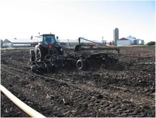
Figure 1. Injection equipment used for pre-plant application (top) and sidedress application (bottom) of liquid dairy manure.
Manure is a valuable source of nitrogen (N) for crop production, but gaseous losses of manure N as ammonia (NH3) and nitrous oxide (N2O) reduce the amount of N available to the crop and, therefore, its economic value as fertilizer. These N losses can also adversely affect air quality, contribute to eutrophication of surface waters via atmospheric deposition, and increase greenhouse gas emission. And the decreased available N in manure reduces the N:P ratio and can lead to a more rapid build-up of P in the soil for a given amount of available N. The most common approach to controlling NH3 volatilization from manure is to incorporate it into the soil with tillage or subsurface injection, which can reduce losses by 50 to over 90% compared to surface application (Jokela and Meisinger, 2008). Injecting into a growing corn crop at sidedress time offers another window of time for manure application (Ball-Coelho et al., 2006). While amounts of N lost as N2O are usually small compared to NH3, even low emissions can contribute to the greenhouse effect because N2O is about 300 times as potent as carbon dioxide in its effect on global warming (USEPA, 2010). We carried out a 4-year field experiment to evaluate the effect of dairy manure application method and timing and time of incorporation on a) corn yield, b) fertilizer N credits, c) ammonia losses, and) nitrous oxide emissions.
What Did We Do?
Figure 2. Average (2009-2011) NH3-N emission rates as affected by method and timing of manure application.
This field research was conducted at the Univ. of Wisconsin/USDA Agricultural Research Station in Marshfield, WI, on predominantly Withee silt loam (Aquic glossudalf), a somewhat poorly drained soil with 0 to 2% slope. Dairy manure was applied either at pre-plant (mid- to late May) or sidedress time (5-6-leaf stage). Pre-plant treatments were either injected with an S-tine injector (15-inch spacing; Fig. 1) or incorporated with a tandem disk immediately after manure application (< 1 hour), 1-day later, or 3 days later. All plots were chisel plowed 3 to 5 days after application. Sidedress manure applications were either injected with an S-tine injector (30-inch spacing) or surface applied (Fig. 1). Fertilizer N was applied to separate plots at pre-plant at rates of 0, 40, 80, 120, 160, and 200 lb/acre as urea and incorporated with a disk. Liquid dairy manure (average 14% solids) was applied at a target rate of 6,500 gal/acre. Manure supplied an average of 158 lb total N and 62 lb NH4-N per acre, but rates varied across years and application times.
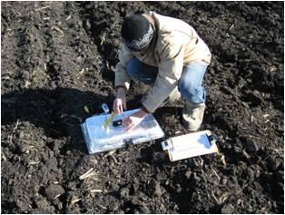
Ammonia emission was measured following pre-plant and sidedress manure applications in 2009-2011 with the dynamic chamber/equilibrium concentration technique (Svensson, 1994). Measurement started immediately after manure application and continued through the third day. Ammonia measurement ended just before disking of the 3-day incorporation treatment, so the 3-day treatment represents surface-applied manure. Nitrous oxide was measured using the static, vented chamber technique following the GRACEnet protocol (Parkin and Venterea, 2010). Measurement began two days after pre-plant manure application and continued approximately weekly into October.
What Have We Learned?
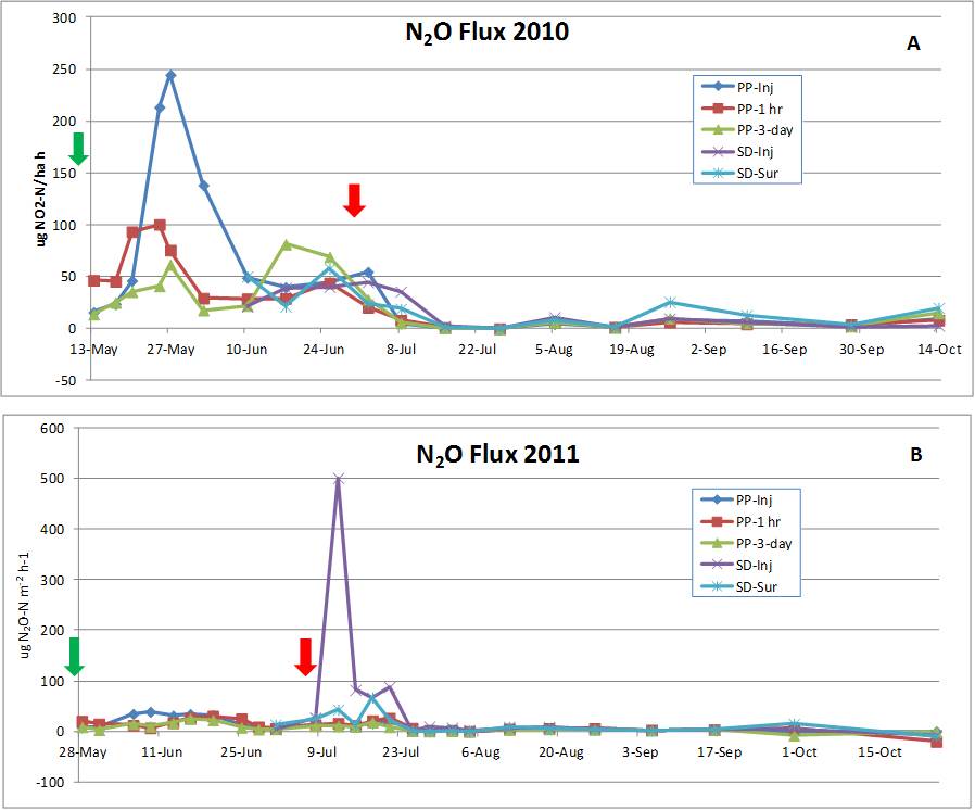
Figure 3. Nitrous oxide (N2O) flux as affected by method and timing of dairy manure application from May to October of 2010 (A) and 2011 (B). Arrows show times of manure application. Note differences in scale for 2010 and 2011.
The 3-year average annual NH3 emission rate from surface applied (3-day incorporation) manure was relatively high immediately following application but declined rapidly after the first several hours to quite low levels (Fig. 2). Cumulative NH3-N loss over the full measurement period averaged over 40 lb/acre from surface application but was reduced by 75% with immediate disking and over 90% by injection. Ammonia losses varied somewhat by year, but patterns over time and reductions by incorporation were similar. The pattern of ammonia loss, 75% of the total loss in the first 6 to 12 hours, emphasizes the importance of prompt incorporation to reduce losses and conserve N for crop use.
Nitrous oxide flux was quite low for most manure treatments during most of the May to October period in both years (Fig. 3). However, there were some increases in N2O flux after manure application, and pronounced peaks of N2O emission from the injection treatment at either pre-plant (2010) or sidedress (2011) time. Greater emission from injection compared to other treatments may have occurred because injection of liquid manure places manure in a relatively concentrated band below the surface, creating anaerobic (lacking in oxygen) conditions. Nitrous oxide is produced by denitrification, a microbial process that is facilitated by anaerobic conditions. Reasons for the difference between 2010 and 2011 are not readily obvious, but are probably a result of different soil moisture and temperature conditions.
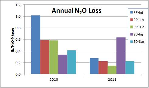
Figure 4. Annual (May-Oct.) loss of N2O as affected by method and timing of liquid dairy manure application. 2010 and 2011.
Based on these results, injection of liquid dairy manure resulted in opposite effects on NH3 and N2O emission, suggesting a trade-off between the two gaseous N loss pathways. However, the total annual N losses from N2O emissions (1 lb/acre or less; Fig. 4) were only a fraction of those from ammonia volatilization, so under the conditions of this study N2O emission is not an economically important loss. As noted earlier, however, N2O is a potent greenhouse gas, so even small amounts can contribute to the potential for global climate change. The dramatic reduction in NH3 loss from injection, though, may at least partially balance out the increased N2O because 1% of volatilized N is assumed to be converted to N2O (IPCC, 2010). Immediate disk incorporation was almost as effective as injection for controlling NH3 loss and, on average, resulted in less N2O emission than injection. But the separate field operation must be done promptly after manure application to be effective. A possible alternative is to use sweep injectors or other direct incorporation methods that place manure over a larger volume of soil and/or create more mixing with soil, thus creating conditions less conducive to denitrification and N2O loss.
Manure application timing and method/time to incorporation significantly affected grain yield in 2009, 2010, and 2012 and silage yield in 2012. Pre-plant injection produced greater yields than one or more of the broadcast treatments in 2009 (grain) and 2012 (grain and silage). Overall, yield effects of application and incorporation timing were variable from year to year, probably because of differences in weather and soil conditions and actual manure N rates applied. The fertilizer N equivalence of manure was calculated by comparing the yield achieved from each manure treatment to the yield response function from fertilizer N. Fertilizer N equivalence values were quite variable by year, but 4-year averages expressed as percent of total manure N applied were 52% for injection (pre-plant and sidedress), 37% for 1-hour or 1-day incorporation, and 34% for 3-day incorporation. So, when expressed as a percent of total manure N applied, N availability generally decreased as time to incorporation increased, which reflects the amounts of measured NH3 loss.
In summary, ammonia volatilization losses increased as the time to incorporation of manure increased. Injection of manure resulted in the lowest amount of NH3 volatilization, but higher N2O emissions. In this study, reducing the large NH3 losses by injecting manure provided more environmental benefit compared to the small increase in N2O emissions. In addition, injection or immediate incorporation resulted, on average, in higher fertilizer N value of manure for corn production. The decreased need for commercial fertilizer N could potentially result in greater profitability and a smaller carbon footprint.
Future Plans
We have started other research to evaluate yield response, N cycling, and emission of NH3 and N2O from various low-disturbance manure application methods in silage corn and perennial forage systems.
Authors
Bill Jokela, Research Soil Scientist, USDA-ARS, Dairy Forage Reserch Center, Marshfield, WI, bill.jokela@ars.usda.gov
Carrie Laboski, Assoc. Professor, Dept. of Soil Science, Univ. of Wisconsin
Todd Andraski, Researcher, Dept. of Soil Science, Univ. of Wisconsin
Additional Information
Ball Coelho, B.R., R.C. Roy, and A.J. Bruin. 2006. Nitrogen recovery and partitioning with different rates and methods of sidedressed manure. Soil Sci. Soc. Am. J. 70:464–473.
Intergovernmental Panel on Climate Change (IPCC). 2006 IPCC Guidelines for National Greenhouse Gas Inventories, vol. 4, Agriculture, Forestry and Other Land Use, edited by S. Eggleston et al., Inst. for Global Environ. Strategies, Hayama, Japan.
The authors gratefully acknowledge Matt Volenec and Ashley Braun for excellent technical assistance in conducting this research. Funding was provided, in part, by the USDA-Agricultural Research Service and the Wisconsin Corn Promotion Board.
The authors are solely responsible for the content of these proceedings. The technical information does not necessarily reflect the official position of the sponsoring agencies or institutions represented by planning committee members, and inclusion and distribution herein does not constitute an endorsement of views expressed by the same. Printed materials included herein are not refereed publications. Citations should appear as follows. EXAMPLE: Authors. 2013. Title of presentation. Waste to Worth: Spreading Science and Solutions. Denver, CO. April 1-5, 2013. URL of this page. Accessed on: today’s date.
Much of the greenhouse gases (GHG) generated from the poultry industry is primarily from feed production. The poultry producer does not have control over the production and distribution of the feed used on the farm. However, they can control other emissions that occur on the farm such as emissions from the utilization of fossil fuels and from manure management. A series of studies were conducted to evaluate on-farm greenhouse gas emissions from broiler, breeder and pullets houses in addition to an in-line commercial layer complex. Data was collected from distributed questionnaires and included; the activity data from the facility operations (in the form of fuel bills and electricity bills), house size and age, flock size, number of flocks per year, and manure management system. Emissions were calculated using GHG calculation tools and emission factors from IPCC. The carbon dioxide, nitrous oxide and methane emissions were computed and a carbon footprint was determined and expressed in tonnes carbon dioxide equivalents (CO2e).
The results from the study showed that about 90% of the emissions from the broiler and pullet farms were from propane and diesel gas use, while only 6% of the total emissions from breeder farms were from propane and diesel gas use. On breeder farms, about 29% of GHG emissions were the result of electricity use while the pullet and broiler farms had only 3% emissions from electricity use. Emissions from manure management in the layer facility were responsible for 53% of the total emission from the facility, while electricity use represented 28% of the total emissions. The results from these studies identified the major sources of on-farm of GHG emissions. This will allow us to target these areas for abatement and mitigation strategies.
Why Study Greenhouse Gases on Poultry Farms?
Human activities, including modern agriculture, contribute to greenhouse gas (GHG) emissions (IPCC, 1996). Agriculture has been reported to be responsible for 6.3% of the GHG emissions in the U.S., of this 53.5% were a result of animal agriculture. Of the emissions from animal agriculture, poultry was responsible for only 0.6%. Much of the CO2e that is generated from the poultry industry is primarily from feed production, the utilization of fossil fuels and manure management (Pelletier, 2008; EWG, 2011). While the poultry producer does not have control over the production of the feed that is used on the farm, there are other GHG emissions that occur on the farm that are under their control. These emissions may be in the form of purchased electricity, propane used for heating houses and incineration of dead birds, diesel used in farm equipment which includes generators and emissions from manure management.
What Did We Do?
A series of studies were conducted to examine the GHG emissions from poultry production houses and involved the estimation of emissions from; broiler grow-out farms, pullet farms, breeder farms from one commercial egg complex. Data collection included the fuel and electricity bills from each farm, house size and age, flock size and number of flocks per year and manure management. The GHG emissions were evaluated using the IPCC spreadsheets with emission factors based on region and animal type. We separated the emissions based on their sources and determined that there were two main sources, 1. Mechanical and 2. Non-mechanical. After we determined the sources, we looked at what contributed to each source.
What Have We Learned?
When all GHG emissions from each type of operation was evaluated, the total for an average broiler house was approximately 847 tonnes CO2e/year, the average breeder house emission was 102.56 tonnes CO2e/year, pullet houses had a total emission of 487.67 tonnes CO2e/year, and 4585.52 CO2e/year from a 12 house laying facility. The results from this study showed that approximately 96% of the mechanical emissions from broiler and pullet houses were from propane (stationary combustion) use while less than 5% of these emissions from breeder houses were from propane use. The high emission from propane use in broiler and pullet houses is due to heating the houses during brooding and cold weather. Annual emissions from manure management showed that layer houses had higher emissions (139 tonnes CO2e/year) when compared to breeder houses (65.3 tonnes CO2e/year), broiler houses (59 tonnes CO2e/year) and pullet houses (61.7tonnesCO2e/year). Poultry reared in management systems with litter and using solid storage has relatively high N2O emissions but low CH4 emissions.We have learned that there is variability in the amount of emissions within each type of poultry production facility regardless of the age or structure of houses and as such reduction strategies will have to be tailored to suit each situation. We have also learned that the amount of emissions from each source (mechanical or non-mechanical) depends on the type of operation (broiler, pullet, breeder, or layer).
Future Plans
Abatement and Mitigation strategies will be assessed and a Poultry Carbon Footprint Calculation Tool is currently being developed by the team and will be made available to poultry producers to calculate their on-farm emissions. This tool will populate a report and make mitigation recommendations for each scenario presented. Best management practices (BMP) can result in improvements in energy use and will help to reduce the use of fossil fuel, specifically propane on the poultry farms thereby reducing GHG emissions, we will develop a set of BMP for the poultry producer.
Authors
Claudia. S. Dunkley, Department of Poultry Science, University of Georgia; cdunkley@uga.edu
Brian. D. Fairchild, Casey. W. Ritz, Brian. H. Kiepper, and Michael. P. Lacy, Department of Poultry Science, University of Georgia
The authors are solely responsible for the content of these proceedings. The technical information does not necessarily reflect the official position of the sponsoring agencies or institutions represented by planning committee members, and inclusion and distribution herein does not constitute an endorsement of views expressed by the same. Printed materials included herein are not refereed publications. Citations should appear as follows. EXAMPLE: Authors. 2013. Title of presentation. Waste to Worth: Spreading Science and Solutions. Denver, CO. April 1-5, 2013. URL of this page. Accessed on: today’s date.
A new method was used at the Ag 450 Farm Iowa State University (41.98N, 93.65W) from October 24, 2012 through December 14, 2012 to assess GHG emission from land-applied swine manure on crop land. Gas samples were collected daily from four static flux chambers. Gas method detection limits were 1.99 ppm, 170 ppb, and 20.7 ppb for CO2, CH4 and N2O, respectively. Measured gas concentrations were used to estimate flux using four different models, i.e., (1) linear regression, (2) non-linear regression, (3) non-equilibrium, and (4) revised Hutchinson & Mosier (HMR). Sixteen days of baseline measurements (before manure application) were followed by manure application with deep injection (at 41.2 m3/ha), and thirty seven days of measurements after manure application.
Static flux chamber (pictured) method was developed to measure greenhouse gas emissions from land-applied swine manure from a corn-on-corn system in central Iowa in the Fall of 2012. Gas samples were collected in vials and transported to the Air Quality Laboratory at Iowa State University campus.
Why Study Greenhouse Gases and Land Application of Swine Manure?
Assessment of greenhouse gas (GHG) emissions from land-applied swine manure is needed for improved process-based modeling of nitrogen and carbon cycles in animal-crop production systems.
What Did We Do?
We developed novel method for measurement and estimation of greenhouse gas (CO2, CH4, N2O) flux (mass/area/time) from land-applied swine manure. New method is based on gas emissions collection with static flux chambers (surface coverage area of 0.134 m^2 and a head space volume of 7 L) and gas analysis with a GC-FID-ECD.
Baseline (post tilling) greenhouse gas (GHGs) emissions monitoring was followed with swine manure application in the Fall of 2012 (pictured) and about 10 weeks of post-application monitoring of GHGs.
New method is also applicable to measure fluxes of GHGs from area sources involving crops and soils, agricultural waste management, municipal, and industrial waste. New method was used at the Ag 450 Farm Iowa State Univeristy (41.98 N, 93.65 W) from October 24, 2012 through December 14, 2012 to assess GHG emission from land-applied swine manure on crop (corn on corn) land. Gas samples were collected daily from four static flux chambers. Gas method detection limits were 1.99 ppm, 170 ppb, and 20.7 ppb for CO2, CH4, and N2O, respectively.
What Have We Learned?
Measured gas concentrations were used to estimate flux using four different mathematical models, i.e., (1) linear regression, (2) non-linear regression, (3) non-equilibrium, and (4) revised Hutchinson & Mosier (HMR). Sixteen days of baseline measurements (before manure application) were followed by manure application with deep injection (at 41.2 m3/ha), and thirty seven days of measurements after manure application. Preliminary net cumulative flux estimates ranged from 115,000 to 462,000 g/ha of CO2, -4.65 to 204 g/ha of CH4, and 860 to 2,720 g/ha N2O. These ranges are consistent with those reported in literature for similar climatic conditions and manure application method.
Greenhouse gases (GHGs) were analyzed in the Air Quality Laboratory (ISU) using dedicated GHGs gas chromatograph. The picture above shows an example of gas sample analysis for CO2, GH4 and N2O. Each ‘peak’ represents one of the tagget GHGs. Gas concentrations were used in a mathematical model to estimate GHG flux (mass emitted/area/time).
Future Plans
Spring 2013 measurements of GHG flux from land-applied swine manure are planned. The spring study will follow the protocols developed for the Fall 2012 season. Estimates of the Spring and Fall GHG flux will be used to develop GHG emission factors for emissions from swine manure in Midwestern corn-on-corn systems. Emission factors will be compared with literature data.
Authors
Dr. Jacek Koziel, Associate Professor, Iowa State University Department of Agricultural and Biosystems Engineering koziel@iastate.edu
Devin Maurer, Research Associate, Iowa State University Department of Agricultural and Biosystems Engineering
Kelsey Bruning, Undergraduate Research Assistant, Iowa State University Department of Civil, Construction and Environmental Engineering
Tanner Lewis, Undergraduate Research Assistant, Iowa State University Department of Agricultural and Biosystems Engineering
Danica Tamaye, Undergraduate Research Assistant, University of Hawaii College of Agriculture, Forestry, and Natural Resource Management
William Salas, Applied Geosolutions
Acknowledgements
We would like to thank the National Pork Board for supporting this research.
The authors are solely responsible for the content of these proceedings. The technical information does not necessarily reflect the official position of the sponsoring agencies or institutions represented by planning committee members, and inclusion and distribution herein does not constitute an endorsement of views expressed by the same. Printed materials included herein are not refereed publications. Citations should appear as follows. EXAMPLE: Authors. 2013. Title of presentation. Waste to Worth: Spreading Science and Solutions. Denver, CO. April 1-5, 2013. URL of this page. Accessed on: today’s date.
The Earth’s climate system is composed of a number of interacting components. The main driver is the sun whose energy is by far the main source of heat for Earth. The sun does not heat the Earth’s atmosphere directly but rather its energy passes through the atmosphere and heats the surface of Earth. The surface then heats the atmosphere from below. If the Earth did not lose heat to space, it would continue to heat up as energy is supplied from the sun. To maintain a fairly constant temperature the Earth must lose as much heat to space as it gains. Clouds, along with naturally occurring carbon dioxide in the atmosphere, prevent some of this heat from escaping and thus warm the Earth. Without these components in the atmosphere the temperature of the globe would be about 60°F colder than it is today. Besides blocking the loss of heat from Earth to outer space, clouds can also reflecting sunlight back to space. This reflected energy is unavailable to heat the Earth.
All of the components of the climate system interact. For example, during ice ages, the growth of ice sheets is triggered by a reduction in the amount of energy reaching the Earth from the sun. As the ice sheets grow, forest and soil covered surfaces, which normally absorb (and therefore are warmed by) solar energy, are replaced by ice. Ice reflects most of the sun’s energy making it unavailable to warm the surface. Therefore the growth of the ice sheets contributes to further cooling of the planet. This is known as a positive feedback, since the cooling due to the reduction in solar energy is enhanced by the ice sheet. The same positive feedback results from global warming, as the extent of the ice sheets diminishes, more soil and potentially forest is exposed. These surfaces absorb more heat than the ice covered areas and hence the warming is enhanced.
Natural forces that effect the climate system
Ice ages are just one example of how the Earth’s climate varies through time. Other variations can be caused by:
Natural fluctuations in the sun’s intensity. The amount of energy emitted by the sun is not constant. Changes in its intensity are typically small (a few tenths of a percent), but can influence temperatures on Earth if they occur over an extended period of time.
Volcanic eruptions. Violent volcanic eruptions like Mt. Pinatubo in 1991 inject sulfur dioxide into the upper atmosphere. This compound is highly reflective to sunlight. Thus its presence in the upper atmosphere prevents a portion of the sun’s energy from reaching the Earth. Once in the upper atmosphere, these compounds can exist for several years following the eruption.
Shorter-term cycles like El Nino. The oceans and atmosphere work together to influence climate. Natural oscillations in ocean currents, the location of the warmest or coldest ocean temperatures, etc. can influence atmospheric circulation patterns. El Nino is an example. In this case the pool of warm water that usually resides in the western tropical Pacific Ocean migrates east. This changes the atmospheric circulation pattern in the tropics which influences global weather patterns.
Human factors affecting the climate system
Increase in greenhouse gases. Carbon dioxide and water vapor are both natural components of the Earth’s atmosphere. These gases, along with methane, nitrous oxide and ozone are termed greenhouse gases (GHGs) because of their ability of absorb some of the energy that the Earth emits to space and reradiate it back to the surface. Prior to industrialization, the Earth’s atmosphere contained about 280 parts per million of carbon dioxide (280 CO2 molecules for every 1,000,000 molecules in the atmosphere). This carbon dioxide was maintained in the atmosphere via volcanic and biological activity.
This graph shows long-term trends in carbon dioxide, the primary anthropogenic (humanmade) greenhouse gas (other greenhouse gases include methane and nitrous oxide). In all but the most recent part of the record the data were obtained from analyzing air samples trapped in
ice cores. Direct measurements have been made since the mid 1950s and fit nicely with the ice core record. Carbon dioxide concentration was very constant prior to 1860. After 1900 the concentrations all increase exponentially.
What causes these increases?
Fossil fuel burning releases about 6 billion tons of carbon each year into the atmosphere.
Methane from agriculture, livestock, landfills and industry has increased by 133%.
Nitrous oxide from agriculture and industry has increased by 15%.
Changes in land use and land cover release 1 billion tons of carbon annually plus other gases.
Land use changes include deforestation and urbanization. Deforestation influences the climate in two ways. 1) Trees are sinks for atmospheric carbon dioxide. They remove CO2 from the air and store it as vegetative matter. Fewer trees mean less CO2 is pulled from the atmosphere. If the trees are subsequently burned, the CO2 is added back to the atmosphere. 2) Removal of the trees changes the character of the land surface; this changes the amount of solar energy that is absorbed by the surface, evaporation, etc. Urbanization is similar to deforestation. Urban areas tend to absorb and hold more heat than vegetated surfaces. Thus cities are typically warmer than rural environments.
Recent Climate Change
When the concentration of greenhouse gases is increased (and everything else in the climate system, like the amount of clouds, is held constant) less of the Earth’s energy escapes to space. As a result the temperature of the Earth must rise.
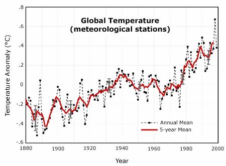
Temperature. Over the last 100 years, instrumental records indicate that the average temperature of the Earth has risen by nearly 1°F (0.5°C). The increases are most pronounced in polar regions of the Northern Hemisphere. In Alaska, temperatures have risen about 2.8°F (1.5°C) over the last century. Across the globe, the increase in temperature tends to be largest in winter, but still significant during the other seasons. Night time temperatures have risen faster than values observed during the day. U.S. temperatures have risen by 0.9°F over the past100 years. Within the past 25 years, U.S. temperatures increased 1.6°F.
Precipitation. Although average precipitation across the globe has not changed dramatically, a change in the character of precipitation has been observed in many parts of the world. The observed trends suggest a shift from more frequent moderate rainfall events to more infrequent heavy rainfall events. Since the period of time between rainfall events increases, drought may become more prevalent. But since the rain events that do occur can be quite heavy, the increased risk of flooding is also a concern. Clearly this change in the character of precipitation has implications for water resource and irrigation decisions.
Predictions
CO2 Levels. In order to project future climate conditions, scientists must predict what the world will look like politically, economically and environmentally in 100 years. Given the uncertainty in such predictions, scientists have developed a range of scenarios of future greenhouse gas emissions. These range from a fossil-fuel intense society that undergoes rapid economic growth and experiences a modest increase in population. In this case atmospheric CO2levels increase to four times their pre-industrial values by 2100. A business-as-usual scenario…continuing the present trend in greenhouse gas emissions … leads to a similar increase in CO2 levels by 2100 (A2 in the figure below).
More environmentally-friendly scenarios, with reductions in fossil fuel usage, also lead to increases in atmospheric CO2 concentration. This results from the lifetime of CO2 in the atmosphere (about 100 years). Thus today’s CO2 emissions are not removed from the atmosphere until 2106. Even the most environmentally friendly emission scenarios lead to an increase in atmospheric CO2 concentration over the next 100 years, to about double preindustrial levels (B1 in previous figure).
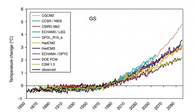
Temperature. Many climate models exist. They all rely on the same physics, but differ in the ways in which variables like clouds are parameterized. The “art” of climate modeling is how processes that can not be well represented by the physics of the models are accounted for. All models experience the same increase in greenhouse gas concentration. They all show a warming by 2100. The only difference is the magnitude of the warming. Here model warming estimates range from 1.5 to 5.0°C by 2100.
Significance. At first glance a degree or two or even five degrees of “global warming” does not seem like a big deal. However when averaged over the globe, this change is quite substantial. From the height of an ice age to the intervening interglacial period (like today) the globe’s temperature changes by about six degrees. The more modest climate model projections are that by 2100, increase global temperature will be about a third of that associated with the ice age cycle. Keep in mind that for ice ages, this six-degree change occurs over 100,000 years. We
expect to see a 2-3 degree change over 100 years!
Precipitation. The figure below shows how precipitation changes will vary geographically by 2100. Some locations (primarily in subtropics) show decreases in precipitation (orange and gold areas in the figure below). Large areas of the middle latitudes and tropics see increases in
precipitation.
Summary
Over the last century the concentration of greenhouse gases in the Earth’s atmosphere has increased markedly. CO2 levels in the atmosphere have not been this high for hundreds of thousands of years. In isolation this change must result in a warming of the Earth’s temperature. Over this same time period climate observations indicate that the global temperature has increased by about 1°F. Although changes in average precipitation have been small (on the order of 1-2%), rain gauge records show that the character of precipitation events has changed. Heavy rainfall events have become more frequent over the last half century.
It is unlikely that the emission of carbon dioxide into the Earth’s atmosphere will slow in the near future. In fact, most projections indicate increased carbon dioxide emissions into the middle to late part of the 21st century. This continued increase will likely lead to additional increases in temperature, with most models projecting rises of between 1.5 and 5°C. Although the exact magnitude of changes in precipitation are uncertain, there is reason to believe that precipitation events will become more variable, leading to increases in both the frequency of floods and droughts.
Manage Cookie Consent
To provide the best experiences, we use technologies like cookies to store and/or access device information. Consenting to these technologies will allow us to process data such as browsing behavior or unique IDs on this site. Not consenting or withdrawing consent, may adversely affect certain features and functions.
Functional
Always active
The technical storage or access is strictly necessary for the legitimate purpose of enabling the use of a specific service explicitly requested by the subscriber or user, or for the sole purpose of carrying out the transmission of a communication over an electronic communications network.
Preferences
The technical storage or access is necessary for the legitimate purpose of storing preferences that are not requested by the subscriber or user.
Statistics
The technical storage or access that is used exclusively for statistical purposes.The technical storage or access that is used exclusively for anonymous statistical purposes. Without a subpoena, voluntary compliance on the part of your Internet Service Provider, or additional records from a third party, information stored or retrieved for this purpose alone cannot usually be used to identify you.
Marketing
The technical storage or access is required to create user profiles to send advertising, or to track the user on a website or across several websites for similar marketing purposes.