w2w22 – Page 5 – Livestock and Poultry Environmental Learning Community

April 20, 2022November 18, 2024

Impact of sampling timing on measured gas concentrations and emissions at a commercial laying hen house

Purpose

Ammonia and carbon dioxide are two major air pollutants at commercial laying hen houses. Ammonia models are widely used to estimate emissions from individual farms, a region, a country, or the world and assess their potential environmental and ecological impacts. Carbon dioxide models have been used to estimate ventilation rates based on mass balance. Reliable models must be developed based on measurement data from field conditions. However, concentrations and emissions of these two gases vary temporally in layer houses and can affect accuracies of measurement data and emission models. Accuracies of the measurement results are largely affected by instruments and methodologies, which includes sampling timing, i.e., number of samples per day (NSPD) and sampling starting time. The purpose of this study is to demonstrate the impact of measurement timing on ammonia and carbon dioxide concentrations and emissions.

What Did We Do?

A dataset of measured gas concentrations and emissions at a commercial laying hen farm was selected and used as a reference. It contains 5 days of continuous measurement data that were saved every minute. Different sampling timing scenarios were selected based on a literature survey and were applied in a computer simulation. Absolute differences in percentage between the simulation results and the reference were used to assess the effects of sampling timing.

Two sampling timing scenarios were used in this study: (a). sampling at eight different NSPD, i.e., 144, 48, 24, 12, 9, 3, 2, and 1 compared with the continues measurement of 1440 NSPD with equal sampling intervals and the first sampling starting at 8:00 AM; and (b). sampling for the same eight NSPD and equal sampling intervals, but with the first sampling starting at six different times within the respective sampling intervals, including 8:00 AM, compared with the data of 1440 NSPD. For example, when the NSPD was 2, the six starting times were selected at 8:00 AM, 10:00 AM, noon, 2:00 PM, 4:00 PM, and 6:00 PM.

What Have We Learned?

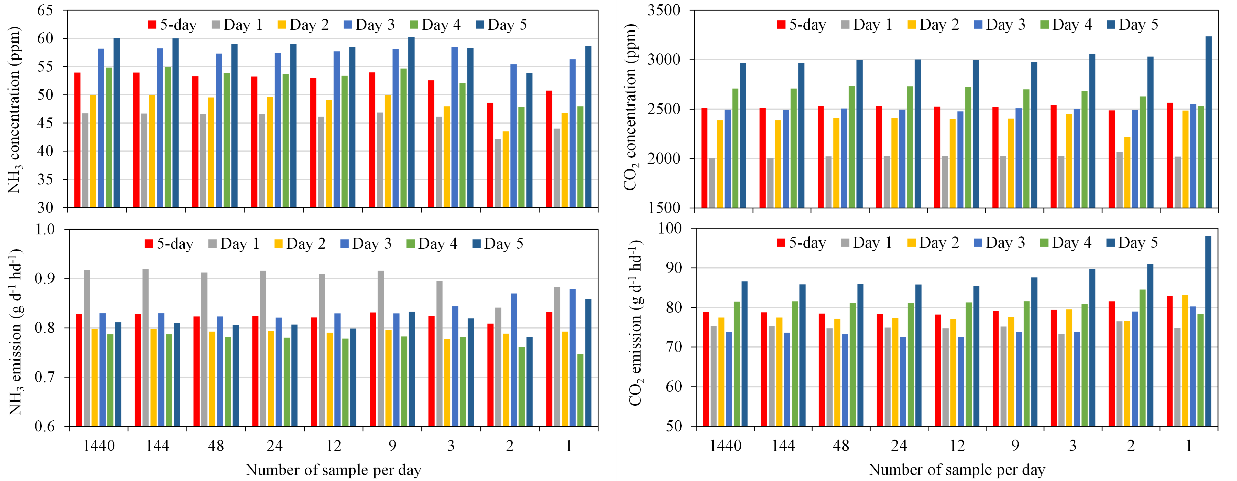
Results demonstrated that, for scenario (a) of the 5 days sampling and measurement (Figure 1), the absolute differences: 1. ranged from 0.02 % (carbon dioxide concentration at 144 NSPD) to 10.04% (Ammonia concentrations at 2 NSPD); 2. was 3.96% for ammonia emissions at 2 NSPD and 6.48% for carbon dioxide emissions at 1 NSPD, both were the largest emission differences; 3. were generally larger in ammonia concentrations than ammonia emissions, but smaller in carbon dioxide concentrations than carbon dioxide emissions; and 4. were generally larger with fewer NSPD for all the four measurement results (ammonia and carbon dioxide concentrations and emissions).

Figure 1. Comparison of average ammonia concentrations (top left), ammonia emission rates (bottom left), carbon dioxide concentrations (top right), and carbon dioxide emission rates (bottom right) with different number of samples per day, starting at 8:00 during a 5-day continuous measurement.

Scenario (b) simulation revealed a new finding that sampling starting times had large impacts on data accuracies as well (Figure 2). The absolute differences 1. ranged from 0.00 % (for both ammonia and carbon dioxide concentrations at 144 NSPD) to 12.92% (ammonia concentrations at 2 NSPD); and 2. was 7.43% for ammonia emissions at 1 NSPD and 7.60% for carbon dioxide emissions at 2 NSPD, both were the largest emission differences. Additionally, scenario (b) demonstrated the same effects as points 3 and 4 in scenario (a).

Figure 2. An example comparison of six different sampling starting times equally distributed within the sampling intervals of 2 hours, at 12 samples per day in the 5 days of sampling on average ammonia concentrations (top left), ammonia emission rates (bottom left) carbon dioxide concentrations (top right), and carbon dioxide emission rates (bottom right).

Future Plans

More research on the effects of sampling timing on gas concentration and emission measurements will be conducted using datasets of longer-term field measurement (> 1 year) with other sampling scenarios based on the literature survey.

Author

Ji-Qin Ni, Professor, Agricultural and Biological Engineering, Purdue University

Corresponding author email address

jiqin@purdue.edu

Additional Information

Wang-Li, L., Q.-F. Li, L. Chai, E. L. Cortus, K. Wang, I. Kilic, B. W. Bogan, J.-Q. Ni, and A. J. Heber. 2013. The National Air Emissions Monitoring Study’s southeast layer site: Part III. Ammonia concentrations and emissions. Transactions of the ASABE. 56(3): 1185-1197.

Ni, J.-Q., S. Liu, C. A. Diehl, T.-T. Lim, B. W. Bogan, L. Chen, L. Chai, K. Wang, and A. J. Heber. 2017. Emission factors and characteristics of ammonia, hydrogen sulfide, carbon dioxide, and particulate matter at two high-rise layer hen houses. Atmospheric Environment. 154: 260-273.

Tong, X., L. Zhao, R. B. Manuzon, M. J. Darr, R. M. Knight, A. J. Heber, and J.-Q. Ni. 2021. Ammonia concentrations and emissions at two commercial manure-belt layer houses with mixed tunnel and cross ventilation. Transactions of ASABE. 64(6): 2073-2087.

Acknowledgements

This work was supported by the USDA National Institute of Food and Agriculture Hatch project 7000907.

The authors are solely responsible for the content of these proceedings. The technical information does not necessarily reflect the official position of the sponsoring agencies or institutions represented by planning committee members, and inclusion and distribution herein does not constitute an endorsement of views expressed by the same. Printed materials included herein are not refereed publications. Citations should appear as follows. EXAMPLE: Authors. 2022. Title of presentation. Waste to Worth. Oregon, OH. April 18-22, 2022. URL of this page. Accessed on: today’s date.

April 20, 2022November 18, 2024

Manure emissions during agitation and processing

Purpose

Recent deaths associated with hydrogen sulfide exposure from manure systems have highlighted the need for increased awareness to reduce health risks. While information on some aspects of hydrogen sulfide release from manure are available, there is limited information on the characteristics when agitating manure storages and in manure processing buildings that result in concentrations that are dangerous to human health. This project aimed to gather data on emissions from manure storages and processing to assess risks and develop mitigation strategies for these risks.

What Did We Do?

Our research team acquired over 20 days of field data (at multiple livestock farms) to assess the air concentrations from manure storages with and without agitation, for hydrogen sulfide, methane, ammonia, and particulate matter. The emissions were measured over the course of eight hours using numerous sets of sensors around the manure storage during agitation for each sampling event. Each sampling event had one backpack that was worn by a researcher with a set of sensors to represent the concentrations relevant to someone working in the area. Five additional sensor sets were placed around the manure storage. Some sensor sets remained in the same position throughout sampling (e.g., at the location of the agitation equipment controls) while others were moved around the storage. Researchers also measured the concentrations of these gases inside a manure processing room to assess the concentration changes with different air exchange rates. During each event manure samples were collected as well as weather data to relate to the manure emissions data.

What Have We Learned?

This research assessed the environmental and design conditions of manure systems that may lead to increased concentrations of gases that have human health implications. The results indicate critical operating parameters on how to manage manure systems to limit risk from gases produced from manure processing and storage areas. More details on the study results will be available soon and will be presented at the conference.

Future Plans

This information is also being integrated into an existing fact sheet, https://learningstore.extension.wisc.edu/collections/manure/products/reducing-risks-from-manure-storage-agitation-gases-p1865, to provide an updated resource which integrates this new data. This information will be shared in a variety of settings to increase awareness and guide practices to reduce health risks to those working with livestock manure.

Authors

Rebecca A. Larson, Associate Professor & Extension Specialist, Biological Systems Engineering, University of Wisconsin-Madison

Corresponding author email address

rebecca.larson@wisc.edu

Additional author

Anurag Mandalika, Assistant Professor, Audobon Sugar Institute, LSU AgCenter

Additional Information

Reducing Risks from Manure Storage Agitation Gases

Acknowledgements

This work is supported by Foundational Program CARE 2019-68008-29829 from the USDA National Institute of Food and Agriculture.

April 20, 2022November 18, 2024

Effects of centrifuges and screens on solids/nutrient separation and ammonia emissions from liquid dairy manure

Purpose

Some Idaho dairies use liquid manure handling systems that result in large amounts of manure applied via irrigation systems to adjacent cropland during the growing season. Solids and nutrients presented in liquid dairy manure pose challenges to manure handling. Separating solids and nutrients from liquid dairy manure is a critical step to improve nutrient use efficiency and reduce manure handling costs. Most Idaho dairies have primary screens that separate coarse particles from their liquid streams. A few dairies have incorporated secondary solid separation technologies (centrifuge and secondary screen) into their manure handling systems to achieve higher solids and nutrient removal rates. Idaho dairymen want to know more information about solid and nutrient separation efficiencies by centrifuges and screens to make informed decisions on upgrading their solid/nutrient separation technologies. The objectives of this study were to evaluate centrifuges and screens in terms of removing solids and nutrients from liquid dairy manure and affecting ammonia emissions from the treated liquid dairy manure.

What Did We Do?

A year-long evaluation of on-farm centrifuges and screens on removing solids and nutrients and affecting ammonia emissions from centrifuge- and screen-separated liquid dairy manure was conducted. Triplicate fresh liquid dairy manure samples were collected monthly from before and after screens and centrifuges on a commercial dairy meanwhile triplicate screen- and centrifuge separated solids were collected from the same dairy. Figure 1 shows the dairy’s liquid manure flow diagram and locations where the liquid and solid manure samples were collected. The collected solids were analyzed for nitrogen (N), phosphorus (P), and potassium (K) concentrations by a certified commercial laboratory. The collected liquid samples were analyzed for total and suspended solids based on Methods 2540B and D (APHA, 2012) in the Waste Management Laboratory at the UI Twin Falls Research and Extension Center. Ammonia emissions from the monthly collected liquid dairy manure were evaluated using Ogawa ammonia passive samplers outside the Waste Management Lab for a year. Ammonia emission rate was calculated based on the duration and NH₄-N concentrations from the Ogawa ammonia passive sampler tests. Ogawa passive ammonia sampler and Quickchem 8500 analysis system are shown in Figures 2 and 3.

Figure 1. Liquid manure flow diagram (liquid manure samples were collected at points 1 (before screens), 3 (after screens), and 5 (after centrifuges), solid samples were collected at points 2 (screen separated solids) and 4 (centrifuge separated solids).

Figure 2. Ogawa ammonia passive sampler.

Figure 3. Quickchem 8500 analysis system (Lachat Instruments, Milwaukee, WI).

What Have We Learned?

Centrifuge can further remove finer particles than cannot be removed by primary screens. Figure 4 shows both the screen- and centrifuge separated solids.

Figure 4. Centrifuge separated (left) and screen (right) separated solids.

Total nitrogen, phosphorus, and potassium in screen- and centrifuge separated solids are shown in Figures 5, 6, and 7. It was noticed that centrifuge separated solids had significantly (P<0.05) higher N, P, and K than that in screen separated solids. Yearlong averages of 9.2 lb/ton of total nitrogen, 8.0 lb/ton of P₂O₅, and 7.2 lb/ton of K₂O were in the centrifuge separated solids while yearlong averages of 5.4 lb/ton of total nitrogen, 2.0 lb/ton of P₂O₅, and 4.4 lb/ton of K₂O were in the screen separated solids.

Figure 5. Total nitrogen in screen separated and centrifuge separated solids.

Figure 6. Phosphorus in screen separated and centrifuge separated solids.

Figure 7. Potassium in screen separated and centrifuge separated solids.

Liquid dairy manure total solids and suspended solids are shown in Figures 8 and 9. Both the total solids and suspended solids in the liquid stream were significantly (P<0.05) reduced after the screen and centrifuge treatment.

Figure 8. Total solids in raw (before screens), after screens, and after centrifuges.

Figure 9. Suspended solids in raw (before the screens), after the screens, and after the centrifuges.

It was found that there was no significant difference (p≥0.05) between treatments for the ammonia emission rate in Figure 10 Which indicates that further treatment is needed to reduce ammonia emissions.

Figure 10. Ammonia emission rate during the test period.

In Figure 11 a correlation was determined between ammonia emission rate and suspended solids. As suspended solids were reduced within liquid dairy manure the ammonia emission rate increased among the treatments.

Figure 11. Ammonia emission rate vs. suspended solids.

In Figure 12 a correlation was determined between ammonia emission rate and ambient temperature. As the ambient temperature increased, so did the ammonia emission rate among the treatments.

Figure 12. Ammonia emission rate vs. suspended solids.

The test results showed:

1. Centrifuge can further remove finer particles that can’t be removed by primary screens.
2. Centrifuge separated solids contained higher N, P, and K contents, especially P (at an average of 8 lb/ton of P₂O₅ in centrifuge separated solids vs. 2 lb/ton of P₂O₅ in screen separated solids).
3. Ammonia emissions from raw liquid manure, screen- and centrifuge separated liquid manure did not show significant differences.
4. The most influential factors for ammonia emissions from liquid dairy manure were ambient temperatures and suspended solids within the liquid dairy manure.

Future Plans

We will hold workshops and field days to communicate the results with producers and promote on-farm adoption of advanced separation equipment such as centrifuge.

Authors

Lide Chen, Waste Management Engineer, Department of Soil and Water Systems, University of Idaho

Corresponding author email address

lchen@uidaho.edu

Additional author

Kevin Kruger, Scientific Aide, Department of Soil and Water Systems, University of Idaho.

Additional Information

APHA. (2012). Standard Methods for the Examination of Water and Wastewater. Washington D.C. : American Public Heath Association., Pp. 2-64 and Pp. 2-66

Acknowledgements

USDA NIFA WSARE financially supported this study. Thanks also go to Scientists at USDA ARS Kimberly Station for their help with analyzing ammonia emission samples.

April 20, 2022November 18, 2024

Does Irrigation of Liquid Animal Manure Increase Ammonia Loss?

Purpose

Large bore traveling gun and center pivot irrigation systems have been used to apply treated lagoon effluent, liquid animal manure, and untreated slurry from swine and dairy farms in many parts of the USA. The primary advantage of using irrigation equipment to spread manure on cropland are the lower costs for energy and labor, and the higher speed of application as compared to using a tractor-drawn spreader. The primary disadvantages are related to increases in odor release and the possibility of spraying manure on roads or another person’s property.

Ammonia-N loss from land application of manure is important because it is a loss of fertilizer nitrogen, and it is a source of air pollution. A previous study and several extension publications state that irrigation of animal manure increases ammonia-N loss by 10% to 25% (Chastain, 2019). As a result, the total ammonia-N loss was the sum of the ammonia-N lost while the manure traveled from the irrigation nozzle to the ground and the ammonia-N lost as the manure released ammonia-N after striking the ground.

The objective of this presentation is to summarize the results of a meta-analysis of 55 data sets from 3 independent sources to quantify the ammonia-N lost during the interval of time from when the liquid manure exited the irrigation equipment and when a sample was collected on the ground. The complete review, data analysis, and the data used were provided by Chastain (2019).

What Did We Do?

The study included data from traveling gun, center pivot, and impact sprinkler irrigation of untreated liquid and slurry manure, lagoon supernatant, and effluent from an oxidation ditch. The data sets included measurements of the total solids content (TS, %), total ammoniacal N concentration (TAN = ammonium-N + Ammonia-N), and total nitrogen (TKN) for a sample collected from the lagoon or storage to describe what was in the manure that left the irrigation nozzle and measurements of the TS, TAN and TKN in the samples that were collected from containers on the ground. The concentrations of TS, TAN, and TKN in the ground collected manure samples were plotted against the TS, TAN, and TKN concentrations in the irrigated manure. The data pairs were analyzed using linear regression to determine if there was a statistically significant difference between the irrigated and ground collected samples. If there was perfect agreement the slope of the line would be 1.0. Therefore, statistical tests were used to determine if the slope of the line was statistically different from 1.0. If the test indicated that the slope was not significantly different from 1.0 then irrigation did not change the concentration of the TS, TAN, or TKN.

What Have We Learned?

Well-known data used in irrigation design indicates that evaporation loss during irrigation ranges from 1% to 3.5%. The plot of the data for irrigated manure is shown in Figure 1. It was determined that the slope of the regression line was statistically greater than 1.0. Therefore, evaporation losses were small, 2.4%, and agreed with previous studies on irrigation performance.

Figure 1. Comparison of the total solids content of the irrigated manure and the samples collected on the ground indicated that evaporation losses were 2.4%.

The plot of the TAN concentrations collected on the ground and the TAN contained in the irrigated water is shown in Figure 2.). The results showed that irrigation of manure did not result in a change in the concentration of TAN. Therefore, irrigation of manure did not cause ammonia-N loss.

The same type of analysis was done for the total nitrogen data to serve as check on the TAN results. As expected, the analysis showed that irrigation did not significantly alter the concentration of TKN.

Figure 2. The concentration of the total ammoniacal nitrogen was not changed as the manure traveled through the air. This was indicated by a regression line slope that was not significantly different from 1.0.

A previous study reported TAN losses ranging from 10% to 25% during irrigation of liquid manure. Error analysis of the techniques used in these studies indicated that most of the average ammonia-N loss predicted was due to volume collection error in the irrigate-catch technique that was used, and not evaporation and drift as was assumed (see Chastain, 2019). It was concluded that irrigation, as a manure application method, did not increase ammonia-N losses. These results do not imply that ammonia volatilization after manure strikes the ground is to be ignored. The suitability of irrigation as a liquid manure application method should be evaluated based on the level of treatment and the potential impact of odors on neighbors.

Future Plans

These results are being used in extension programs and to help refine estimates of ammonia-N loss associated with land application of manure.

Author

John P. Chastain, Professor and Extension Agricultural Engineer, Agricultural Sciences Department, Clemson University

Corresponding author email address

jchstn@clemson.edu

Additional Information

Chastain, J.P. 2019. Ammonia Volatilization Losses during Irrigation of Liquid Animal Manure. Sustainability 11(21), 6168; https://doi.org/10.3390/su11216168.

April 20, 2022November 18, 2024

Estimating Routine Beef and Dairy Mortality Masses Based on Systems Operation

Purpose

The day-to-day loss of animals is a fact of life all cattle producers must face and prepare for. Unfortunately, most published data of animal mortalities are for one-time, catastrophic die offs – where all the cattle on a farm must be exterminated because of disease outbreaks or natural disasters. Routine mortalities on cattle farms do not happen all at once, and mortality rates vary greatly between different life stages of animals and types of production systems.

An expert panel was convened by the Agricultural Working Group of the Chesapeake Bay Program to determine annual mortality, nitrogen and phosphorus masses produced by cow-calf, dairy and cattle on feed (feedlot) operations in the watershed. This paper concentrates on the annual mortality masses estimations determined by the panel. Cattle and Dairymen can use these values to plan for disposal of routine losses.

What Did We Do?

The panel looked, at depth, into existing production systems, and combined morality rates at different life stages, the size of animals at time of death, and the carcass composition varying with age to determine mortality and nutrient masses produced by typical cattle farms in the watershed.

The panel chose a 50-cow cow-calf operation as a model system, where cattle are on pasture 95% of the time. Under ideal conditions, each cow will yield one calf per year to be sold by year’s end. Some female calves will be retained to replace culled cows from the herd, maintaining the same general herd size. It was assumed there was no death loss of mother cows in the herd. We used USDA-APHIS (2010) data of average annual death loss of immature cattle combined with the average weight of cattle at different life-stages to determine weight of mortalities produced each year.

A total confinement beef feedlot was used to model mortalities for cattle on feed. Cattle were assumed to grow linearly with cattle placed in the feedlot at 400 to 600 pounds, and leaving at 1,000 to 1,200 pounds with an average time on lot of 120 days. Midwestern data (Vogel et al, 2015) was used to estimate annual deathrates per feedlot space at 30-day increments since placement in the feedlot.

A 100-cow milking herd was used as a reference for dairy systems. The reference farm contained 50 female calves and 50 heifers in development. Heifers are bred at 15 months and give birth around 24 months (2 years) of age. Male calves are exported from the farm as soon as possible for development as lower grade beef cattle. The reference dairy had heifers and dry cows on pasture, with the active milking herd in free-stall barns or alternative confinement for a 300-day lactation. USDA-APHIS (2016) data of average annual death loss of all types of dairy cattle was combined with the average weight of cattle at different life-stages to determine weight of mortalities produced each year.

What Have We Learned?

Figure 1 shows the estimated total weight of mortalities produced by a 50 cow, cow-calf herd each year broken down by age of animal dying. As can be seen in Figure 1, the greatest weight of mortalities occurred before calves were weaned – assuming no death of mother cows. The values in Figure 1 represent 1.52 calves born dead, 1.92 calves dying before weaning, and 0.87 head dying after weaning. This means a farmer should prepare for the loss of 2 newborn calves, 2 un-weaned calves, and one weaned steer/heifer per 50 mother cows each year. Dividing the total weight of mortalities by 50 head gives an average per cow annual mortality of 32 pounds per year.

Figure 1. Estimated Total Annual Weight of Mortalities Produced by a 50 Cow, Cow-Calf Herd.

Figure 2 shows the estimated total weight of mortalities produced by a 100-head-space feedlot. The greatest source of mortalities is steers and heifers weighing close to 700 pounds (31 to 60 days after arrival on the feedlot. Dividing the total weight of mortalities by 100 gives an average annual mortality weight of 18 pounds per head-space per year. The feedlot owner should prepare for approximately 3 animals dying each year per 100 head-space.

Figure 2. Estimated Total Annual Weight of Mortalities Produced by a 100 head-space feedlot.

Figure 3 shows the estimated total weight of mortalities produced by a 100-cow dairy. Dividing the total weight of mortalities by 100 head gives an average annual mortality weight of 90 pounds per milking cow. The greatest source of mortalities is mature cows. Dairies should prepare for as much as 6 mature cows, 3 pre-weaned calves and heifers, and 1 weaned heifer dying each year per 100 mature cows.

Figure 3. Estimated Total Annual Weight of Mortalities Produced by a 100 milking head dairy.

Future Plans

Cattle producers can use the values estimated by this project to determine resources needed to prepare for mortalities. If burial is the preferred option, the space required to bury mortalities for the expected life of the operation; for composting, the area, and weight of carbon source required to compost; and for incineration, an incinerator capable of handling the largest animal housed on the farm.

Authors

Douglas W. Hamilton, Ph.D. P.E., Extension Waste Management Specialist, Oklahoma State University

Corresponding author email address

dhamilt@okstate.edu

Additional authors

Thomas M. Bass, Livestock Environment Associate Specialist, Montana State University; Amanda Gumbert, PhD., Water Quality Extension Specialist, University of Kentucky; Ernest Hovingh, DVM, PhD., Research Professor Extension Veterinarian, Pennsylvania State University; Mark Hutchinson, Extension Educator, University of Maine; Teng Teeh Lim, PhD, P.E., Extension Professor, University of Missouri; Sandra Means, P.E., USDA NRCS, Environmental Engineer, East National Technology Support Center (Retired); George “Bud” Malone, Malone Poultry Consulting; Jeremy Hanson, WQGIT Coordinator – STAC Research Associate, Chesapeake Research Consortium – Chesapeake Bay Program

Additional Information

Hamilton, D., Bass, T.M., Gumbert, A., Hovingh, E., Hutchinson, M., Lim, T.-T., Means, S., and G. Malone. (2021). Estimates of nutrient loads from animal mortalities and reductions associated with mortality disposal methods and Best Management Practices (BMPs) in the Chesapeake Bay Watershed (DRAFT). Edited by J. Hanson, A. Gumbert & D. Hamilton. Annapolis, MD: USEPA Chesapeake Bay Program.

USDA-APHIS (2010). Mortality of Calves and Cattle on U.S. Beef Cow-calf Operations: Info Sheet, 2010. Fort Collins, CO: USDA-APHIS.

USDA-APHIS. (2016). Dairy 2014: Health and Management Practices on US Dairy Operations, 2014. Report, 3, 62-77. Fort Collins, CO: USDA-APHIS,.

Vogel, G. J., Bokenkroger, C. D., Rutten-Ramos, S. C., & Bargen, J. L. (2015). A retrospective evaluation of animal mortality in US feedlots: rate, timing, and cause of death. Bov. Pract, 49(2), 113-123.

Acknowledgements

Funding for this project was provided by the US-EPA Chesapeake Bay Program through Virginia Polytechnic and State University EPA Grant No. CB96326201

April 20, 2022November 18, 2024

Estimating Routine Swine Mortality Mass based on Systems Operation

Purpose

Swine producers must dispose of the day-to-day losses of hogs and pigs on the farm. Unfortunately, most published data of swine mortalities are for one-time catastrophic events – where all the animals on a farm must be exterminated for disease outbreaks or natural disaster. Routine mortalities on hog farms do not happen all at once, and mortality rates vary greatly between different life stages of swine.

This presentation is the work of an expert panel commissioned by the US-EPA Chesapeake Bay Program to determine annual nitrogen and phosphorus masses produced on swine farms. In this presentation we will show results for annual mortality weights produced on farrow-to-finish, farrow-to-wean, nurseries, and finisher farms.

What Did We Do?

The panel looked, at depth, into existing swine production systems, and combined morality rates at different life stages, size of animals, and the age of varying carcass composition to determine mortality and nutrient masses produced during the production-flow of 25,000 market hogs. All phases of production – gestation, farrowing, nursery, and finishing – rarely occur on the same farm in modern hog production. The panel broke a single farrow-to-finish operation down into its component parts to estimate production of annual mortalities on all types of farms found in the watershed.

What Have We Learned?

Table 1 shows the expected mortality mass produced by a farrow-to-finish swine farm in Southeastern Pennsylvania with a production-flow of 25,000 market hogs per year. Annual Death Rate for all breeding stock (Sows, Gilts, Boars) was assumed to be 7.8% (USDA-APHIS, 2012). Weights at time of death are from Etienne et al. (2016). Weight of Pigs born dead were calculated using values from USDA-APHIS (2012) and Etienne et al. (2016). Mortality masses for growing stock (Weaned Pigs, Feeder Pigs, Finishers) was determined by combining an estimated growth curve for swine (Hamilton et al., 2021) and industry death rate data (Pork Checkoff, 2018). It should be noted that the Pork Checkoff data for mortalities was collected after the PEDv outbreak of the 2010s. Figure 1 shows the cumulative weekly weight of mortalities collected for a population of 1,000 pigs or hogs placed in confinement. It should also be noted that the number of pigs placed in confinement is equal to the number of pigs leaving the previous phase of production in Table 1; i.e., 27,500 weaned pigs entered the nursery each year, 9,600 died in the nursery, and 25,000 left the nursery.

Table 1. Expected annual mass of mortalities and nutrients contained in carcasses produced by a farrow-to-finish operation with a running average of 1,150 sows.
	Inventory	Number Leaving Phase Each Year	Animals Dying (Head yr^-1)	Animal Weight at Death (Lbs.)	Mortality Mass (lbs. yr^-1)
Sows	1,150	–	90	450	40,000
Gilts	115	–	19	300	2,700
Boars	12	–	1	700	700
Pigs Born Dead	0	–	3,200	2.95	9,450
Weaned Pigs	2,000	27,500	9,500	–	30,000
Feeder Pigs	3,900	26,000	1,500	–	64,000
Finishers	9,700	25,000	1,400	–	260,000
Total	16,877				406,900
Per Sow					350
Per Sow Animal Unit					790
Per Finisher Sold					16
Per Finisher Animal Unit					61
Per Inventory Unit					24

Figure 1. Cumulative mass of mortalities measured at the end of each week during the three growth phases of production for groups of 1,000 animals.

Breaking the numbers shown in Table 1 into smaller production units gives the estimated annual production of mortalities for all types of farms (Table 2). It should be noted that the values in Table 2 for Farrow-to-Finish and Farrow-to-Wean farms do not include afterbirth, which can be a major component of biowaste created on farms with farrowing.

Table 2.Estimated Annual Weight of Mortalities Produced by Common Types of Swine Farms.
Annual Weight of Mortalities Produced (lbs. yr^-1)	Farrow to Finish	Farrow to Wean	Off-Site Nursery	Finisher Farm
Per sow	350	73	–	–
Per Sow (1,000 lb. Animal Units)	790¹	160	–	–
Per Pig or Hog Leaving	16	3.0	2.5	10
Per Pig or Hog Leaving (1,000 lb. Animal Unit)	61²	200³	45⁴	39²
Per Feed-Space (Inventory)	24	26	25	27
¹450 lb. sow ²270 lb. Market Hog ³15 lb. Weaned Pig ⁴55 lb. Feeder Pig

Swine producers can use the values estimated by this project to determine resources needed to prepare for mortalities.

Future Plans

Farms raising swine growing stock should size disposal methods based on the highest expected contribution of all additional life stages found on the farm (Figure 1); i.e., ~ 143 pounds per 1,000 hogs per day for finishers, 72 pounds per day per 1,000 nursery pigs. Swine breeding farms should size disposal practices based on the largest breeding head found on the farm, plus the highest expected contribution of all additional life stages found on the farm (Figure 1) plus afterbirth expected on a daily basis. These values are based on conditions in the Chesapeake Bay Watershed, but can be adapted to any locale. For instance, mortalities in the Midwest may be slightly higher because midwestern market weights are slightly higher than those in the Mid-Atlantic Region.

Authors

Douglas W. Hamilton, Ph.D., P.E., Extension Waste Management Specialist, Oklahoma State University

Corresponding author email address

Dhamilt@okstate.edu

Additional authors

Additional Information

Etienne, M., Meinen, R., Kristoff, J., Sexton, T., Long, B., & Dubin, M. (2016). Recommendations to Estimate Swine Nutrient Generation in the Phase 6 Chesapeake Bay Program Watershed Model. Annapolis, MD: Chesapeake Bay Program.

Pork Checkoff. (2018). Checkoff’s Pork Industry Productivity Analysis. Des Moines, IA: National Pork Board. https://www.pork.org/facts/stats/industry-benchmarks/#AverageConventionalFinisherProductivity. Accessed October 1, 2019.

USDA-APHIS. (2012a). Swine 2012 Part I: Baseline Reference of Swine Health and Management in the United States, 2012. Washington, DC: United States Department of Agriculture, Animal and Plant Health Inspection Service. https://www.aphis.usda.gov/animal_health/nahms/swine/downloads/swine2012/Swine2012_dr_PartI.pdf. Accessed June 25, 2019.

Acknowledgements

This project was funded by the US EPA Chesapeake Bay Program through Virginia Polytechnical and State University. EPA Grant No. CB96326201

April 20, 2022November 18, 2024

Estimating Routine Poultry Mortality Masses based on Systems Operation

Purpose

Current design standards and operation guidelines for poultry mortality disposal methods do not adequately account for the non-steady production of carcasses on poultry farms. A common method is to assume poultry die at a constant annual death rate at the mean weight for a placement of birds. While this method may be an accurate estimation for relatively steady-state operations such as egg laying, it grossly overestimates mortality production at the beginning of a grow-out cycle and underestimates mortality production towards the end of a grow-out cycle for meat production operations such as broilers and turkeys.

An expert panel was convened by the Agricultural Working Group of the Chesapeake Bay Program to determine annual mortality, nitrogen and phosphorus masses produced by broiler, turkey, and laying operations in the watershed. This paper concentrates on the mortality masses estimations determined by the panel on a weekly and grow-out basis, using broilers as an example.

What Did We Do?

The weight of mortalities produced each week was determined by combining the expected weekly death rate with growth pattern for broilers. In other words, weight of mortalities collected each week in a grow-out period is equal to number of birds dying during the week times the weight of birds at the time of death. Mortalities collected for an entire grow-out period are then calculated by summing the weekly values. This method can be used to determine mortalities produced for any market weight of bird because market weight is determined by the length of grow-out – all modern commercial broilers having the same basic growth pattern.

What Have We Learned?

Figure 1 illustrates the average growth pattern of broilers using company-provided data for genetic lines commonly used in the Delmarva region. Figure 2 shows weekly mortalities for broilers based on a data set used by the USDA-NRCS in Delaware to design capacity of mortality freezers and industry data provided confidentially to the retired Delaware Extension Poultry Specialist. This death rate data is for antibiotic-free birds. Combining figures 1 and 2 gives the expected weight of mortalities collected by a farmer each week during grow-out per 1,000 broilers placed in a building (Figure 3). Figure 3 shows that weight of mortalities increases each week at an exponential rate with a high degree of correlation (R² = 0.975).

Adding the weight of mortalities collected in one week to those collected in previous weeks gives the total weight collected up to date, or the cumulative weight of mortalities. Since the time required to raise a bird to a certain market weight is known (Figure 1), we can plot the cumulative weight of mortalities during a grow-out period versus market weight of broilers (Figure 4).

The estimated weight of mortalities collected each week and the cumulative weight of mortalities collected over a grow out period can be used to better design and operate mortality disposal methods.

Figure 1. Growth Pattern of Modern Commercial Broilers

Figure 2. Weekly Death Rate of Modern Commercial Broilers

Figure 3. Weight of Mortalities Removed Each Week per 1,000 Broiler Placements

Figure 4. Weight of Mortalities Collected per 1,000 Broiler Placements over One Grow-Out Period for Various Market Weights.

Future Plans

A poultry farmer can use the maximum mass collected each week to accurately size a mortality incinerator or estimate the number of dead birds she will have to cover every day in a mortality composter. Multi-bin composters are usually designed to hold the entire mass of mortalities expected in a grow-out period – plus additional high-carbon and cover material. Designing for this capacity is now possible with an accurate estimate of mortality weight collected per grow-out period.

Authors

Douglas W. Hamilton, Ph.D., P.E., Extension Waste Management Specialist, Oklahoma State University

Corresponding author email address

dhamilt@okstate.edu

Additional authors

Additional Information

Hamilton, D., Bass, T.M., Gumbert, A., Hovingh, E., Hutchinson, M., Lim, T.-T., Means, S., and G. Malone. (2021). Estimates of nutrient loads from animal mortalities and reductions associated with mortality disposal methods and Best Management Practices (BMPs) in the Chesapeake Bay Watershed. Edited by J. Hanson, A. Gumbert & D. Hamilton. Annapolis MD: USEPA, Chesapeake Bay Program (DRAFT).

Acknowledgements

Funding for this project was provided by the US-EPA Chesapeake Bay Program through Virginia Polytechnic and State University EPA Grant No. CB96326201

April 20, 2022November 18, 2024

Thermal Dehydration for the Disposition of Poultry Mortalities

Purpose

In the past 50 years, the poultry industry has made tremendous advancements in production performance, resource utilization and environmental sustainability. However, mortality disposal remains a major challenge as traditional methods of carcass disposal such as burial, incineration, composting, and rendering pose significant risk (biosecurity, environmental pollution, odor, cost, etc.) to the future of the poultry industry.

In North America, approximately 1,500,000,000 pounds of broiler and 187,500,000 pounds of layer hen mortalities must be disposed of in a socially and environmentally sustainable manner without jeopardizing the biosecurity of the production facility nor the financial success of the producer.

What Did We Do

In response to growing concerns and regulatory requirements, an advanced thermal dehydration system has been developed for the disposition of poultry mortalities. This process utilizes simultaneous mixing and heating of the carcass materials in an enclosed drum to 194 F, which results in a 60% reduction in volume over a 12-hour cycle time.

Thermal Dehydration Process

This program was designed to understand the effectiveness, impacts, and opportunities of utilizing Agritech Thermal Disposal Systems thermal dehydration technology for the disposition of poultry mortalities in commercial poultry production facilities in the western United States.

What Have We Learned

Thermal dehydration technology has proven an effective, efficient, and easy method to manage poultry mortalities in commercial poultry production systems. Agritech Thermal Disposal Systems currently offers two models, a smaller single phase unit with a maximum capacity of 1300 pounds and a larger 3 phase unit with a maximum capacity of 2000 pounds per cycle.

The units are simple to operate, as all that is required is to load the mortalities and initiate the thermal dehydration process. There is no requirement for additional materials (carbon), mixing the materials nor manual cleanout, etc.. On average the unit requires 1 kilowatt of electricity per 9 pounds of mortalities processed. An economic analysis comparing thermal dehydration technology with currently used poultry mortality methods is presented below.

Mortality Disposal Comparison
20 Year Analysis
Based on processing 1000 lbs mortality per day
	Rendering	Traditional Incinerator	High Efficiency Dual Burner Incinerator	Rotary Composter	TDS 1300
Fuel Source		LPG	LPG	Wood shavings	Electrical
Amount		2.5 gph	2.5 gph	3:1 ratio	1kW/9 lbs
Fuel per cycle		30 gallons	11.24 gallons	3000lbs	111kW
Cost per cycle	$75	$75	$28	$42.5	$12.5
Cost per week	$526	$525	$197	$298	$88
Cost per year	$27,300	$27,300	$10,238	$15,470	$4,565
Cost per 20 year	$546,000	$546,000	$204,750	$309,400	$91,291
Annual service cost		$1,200	$835	$200	$200
Lifetime Service		$20,400	$15,675	$3,800	$3,800
Replacement time (yr)	5	6.67	20	20	20
Purchase cost	$1,000	$12,000	$32,972	$65,000	$55,000
20 year equipment cost	$5,000	$36,000	$2,972	$65,000	$55,000
500G propane tank		$2,000	$2,000
Building				$75,000	$75,000
Installation cost	$2,500	$2,500	$2,500	$6,000	$3,000
Total investment	$553,500	$606,900	$257,897	$459,200	$148,591
Per lb/cost	$0.076	$0.083	$0.035	$0.063	$0.020
Assumptions
Handling		Carcass handling cost equal
Fuel Cost		2.50$/gallon; 11.30 cents per KWh
Rendering Cost		$0.75 per pound rendering pickup
Woodshavings:		Average 37 lbs/cubic foot
		Utilize 3 cubic yards per day
		1500$/100 yard load delivered ($15/yd)
		Recycle 50% from produced compost
		Plus 30 minutes additional handling per day-20$

Based on industry performance statistics, a 100,000 head broiler facility would produce approximately 3 supersacks/totes of “meat powder” per flock. The resultant “meat powder” is a stable, odor free, sterile byproduct which can be field applied, integrated into commercial fertilizer or utilized in further processing. Compositional analysis has consistently demonstrated a moisture content of approximately 20%, a nitrogen level of 10%, phosphorus of 0.5% and potassium of 0.6%.

“Meat Powder” Produced from Thermal Dehydration Technology

The range in particle size of the resultant “meat powder” was determined through sieve testing in accordance with ANSI/ASAES319, with an average particle size of 560 microns with a standard deviation of 5.06.

Environmental impact analysis of the thermal dehydration process of poultry mortalities has demonstrated that there are no visible emissions from the thermal dehydration unit, other than water vapor.

Further emissions testing has shown total particulate emission rate averaged 0.0066 lb./operating hour, semi-volatile Organic Compounds (SVOCs) were all below the minimum detectable limit and the total combined speciated Volatile Organic Compounds (VOCs) emission rate averaged 0.0067 lb./operating hour, with all individual compounds below regulatory thresholds.

Future Plans

The long-term evaluation program of thermal dehydration technology for the disposition of poultry mortalities continues, with special emphasis on understanding the opportunities to utilize the “meat powder”. These efforts include conducting amino acid profiling, understanding the impacts on quality from long-term storage and determining the optimal handling system.

Thermal dehydration technology has gained international approval for the disposition of animal mortalities, has recently been permitted by the Texas Commission on Environmental Quality and is currently undergoing regulatory review in numerous jurisdictions throughout the United States.

Authors

Jeff Hill, President, Livestock Welfare Strategies
Jeff@LivestockWelfareStrategies.com

Additional Authors

Danny Katz, Agritech Thermal Disposal Systems, Anissa Purswell, Eviro-Ag Engineering, Inc.

Additional Information

www.thermaldisposal.com

Acknowledgements

H and R Agricultural Solutions LLC 1592 Southview Circle Center, Texas 75935

Videos, Slideshows, and Other Media

AgriTech Thermal Disposal Systems – YouTube

April 20, 2022November 18, 2024

Closing the Loop: Evaluating Carcass Compost for Corn Production in Northern Climates

Purpose

Composting is one way that livestock operations can effectively dispose of animal carcasses on their farm site during many times of the year, even in cold climates. Various carbon sources such as wood chips or chopped corn stalks can be used and tend to be coarsely chopped so that airflow is improved through the pile to increase degradation. This makes finished carcass compost different from typical manure or garden compost. Land application is recommended for the final product, but there is little information on nutrient availability of carcass compost for crop production. Since state regulations often require this information to determine appropriate agronomic land application rates, livestock producers are left unable to utilize this material efficiently in a way that meets the law. The goal of this project is to evaluate the fertilizer equivalent value of carcass compost that uses different carbon sources (wood chips versus corn stalks) for corn production.

What Did We Do

The Minnesota Department of Agriculture conducted winter swine carcass composting trials at the University of Minnesota Southwestern Research and Outreach Center in Lamberton, MN during the winter of 2020. In these trials, swine carcasses were ground with the carbon source prior to initiating the compost process. Carbon sources included wood chips or corn stalks. The compost went through the active composting cycles (thermophilic phase) and curing (mesophilic) phase over approximately one year. Samples were collected from each pile in the spring of 2021 and sent to Penn State Analytical Laboratory for standard compost tests.

In 2021, a field experiment was carried out at the University of Minnesota Southwestern Research and Outreach Center in Lamberton, MN to test the different carcass composts as a nutrient source. The field trial was set up as a randomized complete block design with four replications as the blocks. The 10 treatments included:

0 N (full P, K, S) fertilizer (control)
3 urea fertilizer N rates (50%, 100%, 150% of corn nitrogen [N] needs)
3 woodchip compost and 3 corn stalk compost rates (50%, 100%, 150% of corn N needs)

The compost rates were determined assuming 50% of the total N from lab analysis is plant available. The overall N rates were determined using the University of Minnesota fertilizer guidelines for non-irrigated corn. Fertilizers and compost were applied by hand in spring at their appropriate rates and incorporated within 12 hours of application. Approximately 7, 14, and 21 tons per acre of compost were applied to achieve 50%, 100%, and 150% of corn N needs (this corresponds to 80, 160, and 240 pounds of N per acre). Corn was planted and managed for pests according to typical production practices in the region. The middle two rows of each plot were harvested in the fall with a plot combine and yield and grain moisture were recorded.

What Have We Learned

The lab analysis results of each compost are in Table 1. Total N content was similar between sources and primarily made up of organically bound N. The carbon:N ratio of the wood chip compost was higher at 20.8:1 than the corn stalk compost at 14.2:1, though both were below 20:1 and should not theoretically tie up N from the soil after land application. Respirometry tests suggested that the corn stalk compost was not yet mature (respiration was greater than 11 mg CO2-C/g organic matter/day) while the wood chip compost was considered in the “curing” phase (2-5 mg CO2-C/g organic matter/day). The bioassay results suggested that neither compost had any phytotoxins (both had emergence greater than 90%).

Table 1. Swine carcass compost test results from Penn State Analytical Laboratory. Samples were collected and sent to the lab in spring 2021 prior to land application.

	Carcass Compost Carbon Source
Tests	Wood Chips	Corn Stalks
pH	7.3	8.0
Soluble salts (1:5 w:w), mmhos/cm	1.2	2.5
Moisture content, %	29.1	41.2
Organic matter, %	49.1	33.4
Total nitrogen (N), lb ton^-1	22.0	24.0
Organic N, lb ton^-1	22.0	22.0
Ammonium-N, lb ton^-1	0.32	0.66
Nitrate-N, lb ton^-1	0.04	0.00
Carbon: N ratio	20.8	14.2
Phosphorus (as P₂0₅) lb ton^-1	5.4	4.6
Potassium (as K₂0) lb ton^-1	6.6	9.4
Particle Size (<9.5 mm), %	82.6	68.1
Respirometry, mg CO₂C/g organic matter/day	4.8	17.4
Bioassay (cucumber seedling emergence), %	100.0	96.0
Bioassay (cucumber seedling vigor), %	100.0	100.0

As for the field trial, the 2021 growing season endured a sustained drought and yield was lower than expected (ranging from 64 – 117 bushels per acre; Figure 1). Yield increased with each incremental increase in fertilizer N with the highest yield at 240 pounds of N per acre. The carcass composts differed in their effect on yield. Corn yield responded to the corn stalk compost and fertilizer up to 150 pounds of available N per acre (or about 14 tons per acre), but the carcass compost reduced yield at 240 pounds of N per acre. Yield only responded to the wood chip compost at the lowest rate (80 pounds of N per acre, or about 7 tons per acre) but at higher rates yield was similar to the control. This is likely due to the high carbon content of both composts. As more carbon was applied, the soil microbes needed a higher amount of N to degrade the carbon, thus taking it from the soil. Overall, we suggest that less than 15 tons per acre of carcass compost should be used for land application. If wood chips were used as the carbon source, do not expect a significant nitrogen credit.

Figure 1. Corn yield with fertilizer versus swine carcass compost (with either corn stalks or wood chips as the carbon source). Each nutrient source was applied at different rates to supply 80, 160, or 240 pounds of first year available nitrogen. There was also a no-nitrogen control.

Future Plans

We will repeat this study in 2022 at the same site but with compost generated during the winter of 2021. Besides wood chips and corn stalks, a new carbon source will be introduced to the project, wheat straw. Along with yield, we are also evaluating soil and plant samples for nitrogen and phosphorus changes.

Authors

Melissa L. Wilson, Assistant Professor and Extension Specialist, University of Minnesota
mlw@umn.edu

Additional Authors

-Erin L. Cortus, Associate Professor and Extension Engineer, University of Minnesota;
-Paulo H. Pagliari, Associate Professor, University of Minnesota

Acknowledgements

This project is funded by USDA’s Animal and Plant Health Inspection Service through the National Animal Disease Preparedness and Response Program. Thanks to our partners at the Minnesota Department of Agriculture for supplying the carcass compost.

April 20, 2022November 18, 2024

Evaluating Dry Manure Storage Options for Water Quality Protection in Western Washington

Purpose

The purpose of this project was to collect local on-the-ground data to evaluate the effectiveness of different manure storage options installed on working farms in King County, Washington. Agricultural areas in King County receive over 40 inches of rain annually with most of it falling between the months of October through March. During this time, farms often store and compost their manure for spring and summer field application. Composting livestock manure and waste can produce a valuable resource for land managers. However, if managed improperly, manure leachate and runoff can contaminate ground and surface water resources posing a risk to humans and other wildlife.

The project aimed to collect data on water quality and manure quality under different solid manure storage options during the fall and winter months. During the project, we worked with two farms to monitor water quality and manure quality as well as held education and outreach events to engage with stakeholders about benefits and/or costs of adopting new manure management BMPs.

What Did We Do

For the project, we worked with two farms and established four manure storage areas on each including: a concrete slab with walls and a roof, concrete slab with walls and no roof, a compacted soil areas with a tarp cover, and a compacted soil area with no cover. The manure piles were managed by the farmer following common winter practices and were turned and added to 2-3 times per month. We monitored the temperature of the piles over time to assess their composting activity, although it was not a primary focus of our study.

We collected samples of the manure from each storage area during the project to monitor changes over time. To assess nutrient loss and pollution via a stormwater runoff pathway, we collected runoff from the concrete slabs. To assess nutrient loss and pollution via a leaching pathway, we collected soil samples, from under the compacted soil areas. This monitoring allowed us to compare the storage options. The study was conducted over the course of eight months from October 2020 through May 2021. Below are photos of our study setup. Stormwater runoff water quality samples were collected using an ISCO automated sampler that was programmed to grab samples during rain events that generated runoff from the manure piles. Soil and manure samples were collected on a monthly basis.

Figure 1. Manure storage treatments. From left to right: slab covered, slab uncovered, soil covered, and soil uncovered.

Figure 2. Stormwater runoff collection system from the concrete slabs.

What Have We Learned

The project results support the conclusion that the covering of solid manure piles had positive environmental benefits. Covered manure piles stored on a concrete slab have less stormwater runoff with lower loads of nutrients in the leachate than uncovered manure piles on a concrete slab. The covering of dry manure piles stored on compacted soil surfaces reduced the leaching of nutrient, particularly nitrate and nitrite, from manure piles into the soil. It also created a better manure end-product by allowing higher heat values to be reached and creating a drier end product. Additionally, the

placement of manure on a non-permeable, concrete surface eliminated the leaching of manure nutrients below the piles. Covered manure piles, whether stored on a concrete slab or dirt, tended to be drier and have higher temperatures, which results in a better composted manure product.

The results of this study demonstrated that the type of animal species and pile management (how often the pile was turned or added to) also greatly affected the nutrient composition of the leachate. For instance, at Site A, there was higher TP in the manure, and thus higher TP in the runoff water quality and in soil samples.

Future Plans

Due to the short duration of the project, we pursued and were awarded additional funding to extend the project and expand the data set to allow for more robust statistical analysis and conclusions. Partner agencies and organizations as well as the farmers have expressed support and interest in continuing this research, and the project Steering Committee members have also expressed interest in further participation.

In future studies, we intend to try to better quantify the flow volumes from manure piles stored on slabs. In addition, we intend to better assess leaching potential underneath the manure piles stored on soil by using lysimeters to measure leachate volumes.