Dr. Marty Matlock and Dr. Thomas Costello – University of Arkansas
Sub-Project Overview
Algal biomass offers many advantages over traditional energy crops; algal biomass generates higher yields and requires smaller land area than other energy crops. In addition to biomass production for potential biofuel feedstock generation, algal growth systems can also act as tertiary treatment systems for wastewater. Algal growth can dramatically reduce nitrogen and phosphorus from wastewater. Unlike conventional open pond and photo-bioreactor systems, periphytic systems (e.g., algal turf scrubbers) generally involve the polyculture of micro-algae, which does not require specialized conditions. While algal turf scrubber systems are traditionally used for water treatment, they are also capable of generating high biomass yields.
The Algal Nutrient Removal Team has focused on installation of the test bed for the research. This has included construction of a precision graded base for the 20-ft wide by 200-ft long flow way. Our working hypothesis is that operation of an algal flow-way to treat swine manure will remove nutrients, produce a harvestable biomass residue, and add dissolved oxygen which will decrease potential for nitrous oxide emissions (and possibly methane emissions) during manure storage. Wastewater from the swine finisher unit at the University of Arkansas will provide nutrient input to the Algae Flow-way. The flow way will be tested with manure output from pigs fed conventional diets as well as the custom rations intended to reduce manure nitrogen. Impacts on nutrient removal and algal biomass productivity, as a function of diet formulation, will be measured. Nutrient removal will be documented and data collected will be used in the DNDC model to represent the waste treatment performance of the algal systems
Algal growth systems not only provide a method for nutrient removal from animal waste, but also provide biomass production as feedstock for biofuels which can improve the carbon footprint of swine production and other animal production systems in the U.S. This project will provide field scalable data on life cycle impacts of the technology. Design and construct algal turf scrubber concluded in late summer of 2012, and the system is currently undergoing callibrations in preperation for full-scale trials.
Sub-Project Objectives
Measure algal productivity.
Quantify impact of algal nitrogen uptake on swine system GHG emissions.
Dr. Thomas Costello tac@uark.edu
Phone: (479) 575-2847
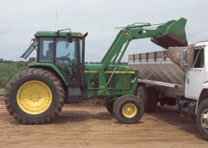
Solids Separation
Dr. Karl VanDevender – University of Arkansas. Cooperative Extension Service
Sub-Project Overview
Many technologies being considered incorporate some type of manure separation to concentrate manure solids, nutrients, and energy content. An LCA study in Denmark showed that energy recovery (incineration, gasification, and anaerobic digestion) had lower GHG emissions than traditional land application of swine manure. Other studies point to the complexities of manure management system design options in relation to GHG emissions. This portion of the project will quantify the effect of various solid separation approaches on the chemical composition of the manure generated by the feed trials at the University of Arkansas facilities during this project ,and generate the necessary manure solids for the thermo-chemical conversion portion of this project. Design and construct a pilot scale mobile solids separation system (see image below) is currently approaching completion and anticipated to be ready to begin trial calibrations soon.
Sub-Project Objectives
Capture and separation of manure from the UA animal experiments.
This unit contains systems to allow for various combinations of mechanical screen and filter bag separation, with and without chemical treatment; and is designed to operate in a batch mode with a capacity of 1000 gallons per batch.
Determine overall characteristics for the feed trial manure samples to provide additional validation data for the animal physiology sub-model.
Contact Information
Dr. Karl VanDevender kvan@uaex.edu
Phone: (501) 671-2244
Auger Reactor Gasification
Dr. Sammy Sadaka – University of Arkansas. Cooperative Extension Service
Sub-Project Overview
Due to the high moisture content, it is not economical to transport raw swine manure over long distances. As a result, manure is spread on land close to the source at high application rates. The energy content of dry manure is in the range of 12 to 18 GJ/ton, about half that of coal. In recent years, wet and dry gasification of algal biomass has been investigated by several researchers. Fluidized bed and downdraft gasification of algal biomass showed various challenges due to the nature of algae biomass. An auger gasification system (see image below) developed in the University of Arkansas, Bioenergy Laboratory, may help to simplify the air gasification process for this type of biomass. Algal biomass was gasified using the auger system during preliminary tests. Several improvements to the system took place during the first year to ensure smooth operation. Our long-term goal is to provide technology to convert swine manure and/or algal biomass to biofuel via a continuous gasification process. Energy conversion technology could provide a revenue stream of about $23 billion/year to the livestock industry.
Sub-Project Objectives
Modify the existing gasification unit to handle swine manure and/or algal biomass.
Test the performance of the gasifier
Optimize the operating parameters to maximize producer gas quality.
Study the effect of reactor temperature on the process yields (gas, char, and tar), as well as on the process efficiency.
Dr. Charles Maxwell, Dr. Jennie Popp, and Dr. Richard Ulrich – University of Arkansas; Dr. Scott Radcliffe – Purdue University, and Dr. Mark Hanigan – Virginia Tech
Why study crude protein and carbon footprint?
Maximizing feed grade amino acid (FGAA) use and reducing dietary crude protein in swine diets has been shown to dramatically reduce nitrogen excretion in both nursery and growing/finishing swine which could substantially reduce nitrous oxide (N2O) emissions associated with manure management in swine production. The global warming potential of N2O is about 298 times that of CO2 (carbon dioxide). Reducing the crude protein (CP) content of grower and finisher diets has also been repeatedly shown to enhance carcass quality by elevating intramuscular fat. While some crystalline amino acids are already commonly used in pork production the maximum level of CP reduction, in conjunction with the optimum amino acid inclusion rate, has not been sufficiently determined for widespread acceptance by the swine industry.
Project Objectives:
Hypothesis: Reducing dietary CP while maintaining amino acids (AA) at equivalent Standardized Ileal Digestibility (SID) ratios by supplementing feed grade AA will reduce nitrogen (N) excretion and greenhouse gas (GHG) emissions (N2O from manure) without impacting swine performance or carcass yield.
Determine the practical limits of reducing CP in diets of nursery and finishing pigs.
Validate the effectiveness of reduced dietary nitrogen as a mitigation strategy for greenhouse gases.
Provide data for validation of animal physiology model capable of predicting swine performance and relevant manure characteristics (quantity and composition for Manure DNDC).
Compare ME vs. NE formulation strategies on lean tissue deposition and fat accretion.
Determine the impact of dietary amino acid levels on signaling in regulation of tissue growth.
[2014 & 2015 annual reports indicated another objective was added] Estimate manure reductions in N excretion via a N balance trial.
Studies were conducted at multiple sites. One was the University of Arkansas wean-to-finish facilities and the second at the Purdue Swine Environmental Research Building (SERB). See the videos above for more on these facilities). The data generated was utilized in modelling work at Virginia Tech. The model was ultimately incorporated into the Swine Environmental Footprint Calculator.
Nursery Studies
What Did We Do? (Methods or Experimental Design)
Experiment 1
To evaluate maximum replacement of CP with FGAA, 320 weaned pigs were allotted to gender-balanced pens in a wean-to-finish facility (8 pigs/pen). Within blocks, pens were randomly assigned to 1 of 5 dietary treatments. Diets were formulated to maintain constant ME and SID Lys across treatments with SID Lys set at 95% requirement (PIC Nutrient Specification Manual, 2011). Diets were formulated to meet the SID AA ratio recommendations for other indispensable AA (SID) for nursery pigs through the 6th limiting AA (PIC Nutrient Specifications Manual, 2011). For each phase, Ctrl diets were devoid of FGAA, whereas Lys HCl was added in equal increments at the expense of CP (SBM, fish meal [FM], and poultry meal [PM] in phase 1, FM and PM in phase 2, and SBM in phase 3). This formulation procedure resulted in diets that were below the His and Phe/Tyr SID requirement for the highest level of CP reduction. CP and Lys inclusion levels were analyzed. Experiment 2
A second three phase nursery study was conducted with pigs weaned at 21 d to further evaluate limits of CP reduction in nursery diets and compare performance in pigs fed diets based on formulation on an ME vs. NE basis. The study involved 7 pigs/pen and 7 replicates/treatment. Dietary ingredients were similar to those used in experiment 1, except soy protein concentrate was used to replace fish meal. Dietary treatments were: 1), Control diet formulated on an ME basis and with FGAA used to meet the “Trp Set Point” without adding feed grade Trp in phase 1 and 2 and 0.02 % added Trp in phase 3; 2) Diet formulated on an ME basis and to meet the “His Set Point” without added feed grade His; 3) As 2 with diets formulated on a NE basis.
Nursery What Did We Learn (Results)?
Experiment 1
Pigs fed RCP 1, RCP 2, and RCP 3 diets in phase 1, 2 and 3, and for the overall study had similar ADG and BW but growth performance declined for pigs fed RCP 4 diets (Table 5; Quadratic effect, P < 0.01). A similar response was observed in ADFI in all time periods except phase 1 where ADFI was similar among treatments. In phase 1, G:F ratio followed a similar response (Quadratic effect, P < 0.01), but decreased linearly in phase 2 (P < 0.08), 3, and overall (P < 0.01). It should be noted that the RCP 4 diet was below requirement for SID His:Lys and Phe/Tyr:Lys which might explain the decrease in performance. The results of this study establishes that a high inclusion of feed grade Lys at the expense of intact proteins can be fed without decreasing ADG and ADFI except at the highest level of FGAA where the requirement for all IDAA was not met. However, G:F was generally reduced at the higher inclusion rates of FGAA, particularly in phase 3. Experiment 2
No differences were observed in ADG, ADFI, or G:F (Table 6) in any phase or overall in pigs fed diets formulated on an aggressive FGAA inclusion (His Set Point) based on ME (Trt.2) or NE (Trt. 3) compared to pigs fed AA inclusion levels currently used in swine industry (Trt. 1). These results indicate that in nursery pigs, one should be able to use a His Set Point in formulating AA based diets without concern for pig performance.
The previous nursery experiment (Experiment 1; Bass et al., 2013) conducted to evaluate feeding reduced CP diet with the highest levels of FGAA to nursery pigs resulted in poor growth performance, especially G:F ratio in phase 3 and the overall nursery period. In the previous study, experimental diets were formulated to meet the 95% of SID Lys requirement for nursery pigs. Also, RCP 4, which was formulated with the highest level of FGAA, did not meet the His and Phe requirement Lys/NE.
Conclusion
In conclusion, unlike the previous study, growth performance of nursery pigs was not affected by the higher level of FGAA and lower dietary CP. This may be due to different SID His:Lys and SID Phe+Tyr:Lys ratios used in diet formulation or different protein source used in each study. In the second nursery study, all diets were formulated based on 100 % or excess of SID Lys requirement for nursery pigs, and were formulated to meet the His and Phe+Tyr requirement. In addition, soy protein concentrate (SPC) was used in the second study during phase 1 and 2, replacing menhaden fish meal used in nursery study one.
Publications
2013 Midwest American Society of Animal Science (ASAS) meeting (Experiment 1) Abstract P042, page 102
Grow-Finish Studies
What Did We Do? (Methods)
Each experiment was conducted following a five phase grow-finish protocol. Pigs were fed 1 of 4 or 5 diets and 10 ppm of Paylean was fed during the final 3-week finishing phase-Phase 5. During phase 1 through 5, individual pig BW, and pen feed disappearance were measured over each phase to allow calculation of ADG, ADFI and G:F by phase. Tenth rib, ¾ midline back fat measurements and loin muscle area were estimated at study initiation and at the end of each phase via ultrasound to allow estimation of carcass lean gain. When the average of all blocks was 129-134 kg all pigs were individually weighed, tattooed, transported to, and harvested at a commercial pork packing plant according to industry accepted procedures. Longissimus muscle (LM) and fat depths at the 10th rib were measured on-line with a Fat-O-Meater probe and individual hot carcass weight was recorded. Experiment 1
A total of 420 pigs were blocked within gender and randomly allotted to pens with 6 pigs/pen. Within blocks, pens of pigs were randomly assigned to 1 of 5 dietary treatments (7 reps/treatment/gender). Diets were formulated by incrementally increasing levels of Lys with corresponding reductions in CP. Pigs were randomly allotted to the following diets:
Ctrl: Corn-SBM-DDGS diets devoid of FGAA,
RCP 1 (reduced crude protein 1)
RCP 2
RCP3
RCP 4 – was balanced on the requirement of the 7th limiting AA, His (PIC Nutrient Specifications Manual, 2011) which was considered the practical limit of the highest level of RCP because of availability constraints.
RCP 1 to 4 were then formulated to have stepwise and equally spaced increased Lys with corresponding reductions in CP between RCP 1 and 4. Diets 2-4 were supplemented with FGAA as needed to meet AA needs based on AA minimum ratios. Dietary CP and Lys inclusion levels were analyzed.
Diets were formulated to 95% of the average SID Lys requirement for barrows and gilts (PIC Nutrient Specifications Manual, 2011), and exceeded the SID AA/Lys ratio recommendations for other IDAA by 2 percentage points.
Distillers dried grains with solubles (DDGS) were included in all diets at the 20% level, with the exception of phase-5 finishing diets which was devoid of DDGS. Experiment 2
In experiment 1, diets were formulated on an ME basis and as soybean meal was reduced in diets, the calculated Lys/NE decreased which may explain some of the increase in fat deposition in pigs fed ME based diets formulated by decreasing soybean meal and including high levels of FGAA. Therefore, experiment 2 was conducted to establish the efficacy of using a “Set Point SID requirement” of sequentially reducing CP by adding FGAA to meet the SID IDAA/Lys ratio as a means of establishing the practical limits of CP reduction and AA replacement without impacting growth performance, carcass composition or quality in growing and finishing pigs fed NE based RCP diets. Diets were formulated starting with a Ctrl diet that approximates acceptable inclusion levels of FGAA currently used in industry, followed by sequentially formulating three additional dietary treatments, each based on the next limiting AA. Diets in this study were formulated on a constant NE basis within phase. DDGS was included in all diets. The SID His requirement in the highest RCP diet was met in each phase without added feed grade His.
There were a total of 9 replicates/treatment with pigs housed 6 pigs/pen. Sex within pen was balanced. Diets were formulated as in experiment 1 which were:
Treatment 1, Ctrl: Conventional phase 1 through 5 diets that approximates acceptable levels of FGAA currently used in industry. The assumption is that most in the industry are comfortable utilizing feed grade Thr and Met to meet the suggested SID Thr/Lys and Met/Lys ratio in diets formulated to meet the SID Trp/Lys requirement without added feed grade Trp. This is referred to as the Trp Set Point.
Treatment 2, RCP 1: Diets were formulated to meet the next limiting AA. In phase 1 and 5, the next limiting AA was Val while Ile was next limiting in phases 2, 3 and 4. This is referred to as the “Val or Ile Set Point”. Note that neither feed grade Val nor Ile were added in any phase.
Treatment 3, RCP 2: Diets were formulated to meet the next limiting AA. In phase 1 and 5, the next limiting AA was Ile while Val was next limiting in phases 2, 3 and 4. This is referred to as the “Val and Ile Set Point”. Note that feed grade Val but not Ile was added in phases 1 and 5, and Ile but not Val was added in phase 2, 3, and 4.
Treatment 4, RCP 3: Diets were formulated to meet the next (7th) limiting AA, His. This is referred to as the “His Set Point”.
All diets were supplemented with FGAA to meet IDAA recommended levels. Note that feed grade His was not added to any diet.
Grow-Finish Studies – What Did We Learn?
Experiment 1
Body weights of pigs decreased linearly with decreasing dietary CP during phase 1, 2, and 3 (P < 0.01; Table 7). Additionally, BW increased and then decreased quadratically during phase 3 (P = 0.09), 4 (P < 0.04), and 5 (P < 0.01) with BW decreasing significantly in pigs fed RCP 4. When Paylean was included in the Phase 5 diets, barrows fed the Ctrl diet had greater ADG than Ctrl-fed gilts, but RCP 1-, RCP 2-, and RCP 3-fed gilts had greater ADG than their castrated male counterparts (Quadratic gender × reduced CP diet, P = 0.08; Figure 1A) Both ADG and G:F decreased linearly (P ≤ 0.06) during phase 1 and 2. Furthermore, gain efficiency increased 4.6 % in gilts between Ctrl and RCP 2 before decreasing to similar G:F values between Ctrl and RCP 4; however, G:F remained relatively unchanged in barrows across the 5 dietary treatments (Quadratic gender × reduced CP diet, P = 0.04; Figure 1B).
Across the entire feeding trial, ADG increased only 2 % between Ctrl and RCP3, but dropped 6 % between RCP3 and RCP4 (Quadratic, P < 0.01). On the other hand, ADFI tended to decreased linearly (P = 0.09) as CP was reduced in swine diets. Gain efficiency increased 4.6 % in gilts between Ctrl and RCP2 before decreasing to similar values between Ctrl and RCP4; however, G:F remained relatively unchanged in barrows across the 5 dietary treatments (Quadratic gender × reduced CP diet, P = 0.04; Figure 1C).
Reducing dietary CP and optimizing the use of FGAA had limited (P ≥ 0.21) effects on HCW, dressing percentage, or LM depth; however, 10th rib fat depth increased linearly (P < 0.01), and fat free lean percentage at study termination decreased linearly as CP was reduced in swine diets (P < 0.02; Figure 1D). Experiment 2
Effects of dietary treatment (Trt.) indicated that ADG decreased linearly with increasing dietary FGAA in phase 3 (Table 8, P < 0.05), 4 (P < 0.10), 5 (P < 0.01) and overall (P < 0.01). Similarly, ADFI decreased linearly in phase 4 (P < 0.05), 5 (P < 0.01) and overall (P < 0.01) with increasing FGAA. Compared to pigs fed the control diet (Trt. 1), G:F in phase 1 increased in pigs fed increasing levels of FGAA at the lower inclusion rates (Trt. 2 and 3) before decreasing to the control level at the highest level of inclusion (Trt. 4, Quadratic effect, P < 0.05). During phase 3, a small, but significant, decrease in G:F was observed with increasing levels of FGAA (Linear effect, P < 0.05). For the overall study, however, a trend for increased G:F was observed (Linear effect, P < 0.06). BW increased at the end of phase 2 with increasing level of FGAA (Quadratic effect, P < 0.06). However, consistent with ADG, BW decreased with increasing dietary FGAA at the end of phase 3, 4 and 5 (Linear effect, P < 0.05, P < 0.01 and P < 0.01, respectively).
As might be expected based on BW, HCW decreased with increasing inclusion of dietary FGAA (Linear effect, P < 0.01). Tenth rib backfat was lower in pigs fed diets formulated to the Val or Ile Set Point (Trt. 2) or the His Set Point (Trt. 4) when compared to those fed diets formulated to the Val and Ile Set Point (Trt. 3).
Publications – G/F (Trial 1)
2013 Midwest American Society of Animal Science (ASAS) meeting Abstract 0224, page 73 (performance and carcass composition)
2013 Midwest American Society of Animal Science (ASAS) meeting Abstract P027, page 97 (LM – longissimus muscle quality)
Significance. This information is timely since the cost of soybean meal is approaching record levels which make substitution of synthetic amino acids for intact protein more economically feasible.
Nitrogen (N) Balance Study
What Did We Do? (Methods)
Thirty-two barrows were used to evaluate the effect of feeding reduced CP, AA supplemented diets, on nutrient and VFA excretion. Pigs were randomly allotted to the following diets:
Control: Corn-SBM-DDGS diets with no FGAA,
1X reduction in CP,
2X reduction in CP, and
3X reduction in CP. This diet was balanced on the 7th limiting AA in each phase.
Diets 2 and 3 were formulated to have stepwise and equally spaced reductions in CP between diets 1 and 4. Diets 2-4 were supplemented with FGAA as needed to meet AA needs based on NRC 2012 AA minimum ratios. Four nursery phases and 5 grow-finish phases (21d phases) were fed. Pigs were housed in stainless-steel metabolism pens equipped with a nipple waterer and stainless steel feeder. Collections started with nursery phase 3 and during nursery phases pigs were allowed an eight day adjustment period to the diets followed by a 3 d total collection of feces, urine, and orts. During the grow-finish phases, pigs were acclimated to diets for the first 10 d of each phase, and then feces, urine, and orts were collected for 3 days.
Nitrogen Balance – What Did We Learn? (Results)
Overall, from d 14-147 post-weaning ADFI was linearly increased as dietary CP was reduced, but no effect of dietary CP concentration on ADG or G:F (Table 9) was observed. Fecal excretion (DM) tended to respond in a quadratic (P = 0.08) fashion with decreasing fecal excretion (DM) up to 2X reduction in CP, but then increasing in 3X fed pigs. Both DE and ME (kcal/kg) were linearly (P < 0.01) reduced as dietary CP was reduced. The linear (P < 0.01) decrease in N intake for pigs fed reduced CP diets was accompanied by linear (P < 0.01) decreases in both urinary and total N excreted. Nitrogen digestibility (%) linearly decreased (P < 0.01) and N retention linearly (%) increased (P < 0.01) with reductions in dietary CP. Overall, there was a linear (P < 0.03) reduction in fecal ammonium as dietary CP was reduced. Total carbon (C) intake and total fecal C excreted tended (P = 0.06) to respond quadratically with an increase in both C intake and C excretion up to the 1X reduced CP diets, followed by a decrease in C intake and increasing C excretion to the 3X diet creating a linear (P < 0.05) decrease in C digestibility as dietary CP was reduced.
Significance. The ability to add total fecal and urine collections of the nitrogen manipulation diets across all body weights tested at the University of Arkansas before the diets were tested for greenhouse gas emissions at Purdue University improved the estimation of compounds excreted in fresh manure and then the conversion of these excreted nutrients and compounds during storage in typical deep pit manure structures under the swine facilities (as were measured during the Purdue 12 room study). This research project provided data for a critical link between excretion, storage, and land application.
Validating the Nursery, Grow-Finish, and GHG Measurement Studies
Large-scale trials are in progress to validate the nursery and grow-finish trials done at Arkansas. The Purdue facility is scaled more similarly to a commercial production system. Gas measurement and monitoring, and separate manure handling systems for each room allowed direct measurements with which to compare previous estimations.
Treatment structure for the experiment was:
Conventional diet containing ~ 0.15% Lys-HCl
1X reduction in CP with additional synthetic amino acids
2X reduction in CP with additional synthetic amino acids
All diets were supplemented with Ractopamine during the final 3-4 weeks of the trial, and amino acid concentrations were increased based on estimated increases in lean tissue accretion. However, the overall treatment structure will remain the same. The Experiment involved 24 pens of 10 pigs each per treatment, with 8 manure pits/trt, and 4 rooms per trt. Pen was the experimental unit for all growth performance, feed intake, and carcass data. Pit was the experimental unit for manure excretion data and room is the experimental unit for emission data.
Real-time monitoring of air temperatures included relative humidity, carbon dioxide (CO2), methane (CH4), nitrous oxide (N2O), ammonia (NH3), and hydrogen sulfide (H2S). Total suspended particulates were monitored using gravimetric samplers. The emission and animal performance data were significantly more accurate in this replicated, environmentally-controlled building than is possible commercially, yet still simulate commercial conditions.
Manure from each pit was completely removed to outside storage for volume determination, thorough agitation and sampling at the end of each trial. In addition, core manure samples based on a grid system were obtained at the end of each growth phase. Manure volume in each pit was determined at diet phase changes by taking 6 gridded depth measurements between the slatted floor. Manure samples were analyzed for pH, dry matter, ash, total nitrogen (N), ammonium N, phosphorus (P), carbon (C), and sulfur (S). Data defining the relationship between the reduction in dietary CP with a reduction in manure N and other changes in manure characteristics are essential to model development of the impact of this mitigation strategy on GHG emissions. An additional benefit will be defining the limits of this strategy without impacting animal growth performance under conditions where industry stakeholders have input.
Validation study – What did we learn (results)?
Coming Soon! (first half 2016)
Modeling the Data
[See also: Virginia Tech modeling efforts] Current nutritional requirement models for swine are focused on partitioning of dietary energy and amino acids to maintenance, growth, gestation, and lactation. Little focus is placed on predicting nutrient excretion, and thus these models cannot be used to provide inputs to an emissions model. Models that predict excretion of energy, protein, and phosphorus have been developed, but have not been evaluated for the accuracy of predictions; and evaluations that have been undertaken focus on predictions of growth and body composition, not nutrient excretion.
GHG emissions from manure storage facilities can be predicted from manure composition, underscoring the need for a robust animal model capable of predicting both animal performance and nutrient excretion. Prediction of GHG emissions from swine manure requires knowledge of N and volatile solids content, neither of which are provided by current NRC predictions.
Data from the nitrogen mitigation growth and nitrogen excretion studies were utilized in enhancement of an animal model capable of predicting swine performance and excretion of nitrogen, carbon, and volatile solids (inputs required by the DNDC model). The growth model developed by the workers at UC-Davis and the recently released Nutrient Requirements of Swine (NRC) eleventh revised edition will be used as a starting point for model development. Equations describing the response to dietary protein and amino acid additions will be evaluated for accuracy, and the effects of Paylean on animal performance and manure nutrient output will be encoded and tested for accuracy. This work is scheduled to precede and utilize data from the UA trial and literature sources. The model will be further evaluated in the 5th year using the Purdue data set.
Why Study Health of Pigs In Relation to Greenhouse Gas (GHG) Emissions?
Our working hypothesis is that immune activation, from clinical and subclinical disease, reduces growth performance and concomitantly increases nutrient excretion and subsequent GHG emissions from manure management.
Findings from this project will provide validated information for incorporation into the animal physiology models.
Project Objectives
Vaccination/PRRSV Trials
Evaluate impact of Porcine Reproductive and Respiratory Syndrome Virus (PRRSV) exposure and vaccination on animal performance, manure output and composition, and greenhouse gas (GHG) emissions from stored manure.
Antibiotics and Antibiotic Alternatives
Evaluate the effects of health status on GHG emissions and carbon and water footprints
Salmonella
Evaluate effects of health status (Salmonella) on animal performance, manure output and composition, and GHG emissions from stored manure.
Research Summary: What Have We Done? What Have We Learned?
Manure reactors installed at Virginia Tech for the pilot study. The manifold on the wall distributes a constant stream of air to each bioreactor, and forces gas through the exhaust lines into the gas analyzers
Thermo Scientific analyzers for carbon dioxide (CO2), methane (CH4), nitrous oxide (N2O), mono-nitrogen oxides (NOx), ammonium (NH4), and hydrogen sulfide (H2S). A programmable manifold switch will sample gas from each reactor sequentially throughout the day.
Vaccination/PRRSV
Experimental Design:
Pigs were randomly assigned to a 2 x 2 factorial design investigating the interaction of Porcine Reproductive and Respiratory Syndrome Virus (PRRSV) vaccination (with or without) and exposure to the PRRSV. One week after weaning, pigs were treated intramuscularly with 2.0 mL of a commercial PRRSV vaccine (Ingelvac PRRS MLV) or sterile saline and housed 4/pen (2 barrows and 2 gilts). Pigs were inoculated 3 weeks after vaccination with sterile medium or PRRSV (MN184). This vaccination protocol has provided high protection against experimental PRRSV infection. (Thacker et al., 2000). Blood samples were collected from pigs upon arrival to the biosafety laboratory to corroborate PRRSV-naïve status. Pigs were given antibiotic-free diets that meet or exceed all nutrient recommendations (NRC, 1998). Growth performance, manure output and composition, and GHG emissions were determined from manure collected from each pen. The study was carried-out for 4 weeks after PRRSV inoculation and used a total of 3 experimental units (i.e., pens) per treatment (i.e., 48 pigs in total). The mitigation strategy tested was the effect of vaccination on pig growth and GHG emissions.
Porcine Reproductive and Respiratory Syndrome Virus (PRRSV) infection caused significant reductions in feed intake which led to reductions in rates of gain and body weight. The infection also caused a reduction in diet digestibility leading to greater manure nutrient output per unit of feed intake and increased greenhouse gas (GHG) production from the stored manure. The impact on GHG production is particularly striking when the data are expressed as litters of gas per kilogram of body weight gain. The increased gas production combined with reduced rates of gain results in more than a tripling of gas production per unit of gain for all of the gases. Vaccination against PRRSV appeared to offer little benefit in terms of animal performance, manure nutrient output, or gas production from manure. Results of the gas production data are presented in Table 1.
Antibiotics and Antibiotic Alternatives
Experimental Design: Seven hundred twenty-four, mixed sex pigs were placed in 11 rooms at the SERB to determine the effects of rearing pigs without antibiotics on growth performance. Pigs were blocked by (body weight) BW and gender and allotted to room and pen with 10/11 mixed-sex pigs/pen. Control pigs consumed diets (Table 2) containing antibiotics and were treated with injectable antibiotics when deemed necessary. Antibiotic-free animals consumed diets with alternatives to antibiotics and received no injectable antibiotics. If sick animals did not respond to antibiotic alternatives, they were removed from the experiment.
Pigs were weighed at the start and end of each dietary phase, and mortality and morbidity were recorded daily. Data were analyzed using the general linear model (GLM) procedure in SAS (statistical software). During the nursery phase, control pigs grew faster (P<0.02; 0.449 vs 0.426 kg/d), and consumed more feed (P<0.05; 0.694 vs. 0.660 kg/d) than antibiotic free animals, resulting in similar (gain to feed ratio) G:F.
Similar average daily gain (ADG), average daily feed intake (ADFI) and G:F were observed throughout the grower phases, and therefore the increased BW of control-fed pigs was maintained and tended (P=0.06) to be heavier at the start of the finisher phases (86.0 vs. 84.5 kg). However, antibiotic-free animals grew 3% faster (P<0.01) and had 6% better G:F (P<0.001) in the finisher phases.
As a result, there was no overall effect (P>0.10) of treatment on ADG, but there was a trend (P = 0.08) for increased ADFI (2.11 vs. 2.07 kg) and reduced (P<0.05) G:F (0.518 vs. 0.527) in control pigs compared to antibiotic-free. Thirty antibiotic-free animals (8.3%) were removed from the study compared to 11 control (3.0%). In conclusion, antibiotic-free management can yield a similar growth performance to conventional systems, but the limited disease treatment options may limit the number of pigs marketed under this management system.
Salmonella Trial
Experimental Design:
The objective of the study was to determine the impacts of a dirty environment leading to increased pathogen load and salmonella infection on animal performance, manure output and composition, and GHG production from the stored manure. 24 3-week old pigs were transported from the VT swine facility to the Biosafety Laboratory on campus and randomly allotted to one of the following health statuses: 1) High (clean room); 2) Medium (replicated clean on-farm environment); 3) Low (replicated “dirty” farm environment); or 4) Low + Salmonella challenge. Pigs were housed in individual metabolism stalls and fed the same antibiotic free diet as for the VT PRRSV trial. All pigs were assessed for fecal salmonella shedding which is indicative of an active infection upon arrival and found to be negative, and the feed was checked for salmonella contamination and found to be negative. After 10 days of adjustment (31 d of age), pigs allotted to the infected group were orally inoculated with 1×10^9 CFU of Salmonella enterica serotype enterica serovar Typhimurium strain DT104 (ATTC; BAA-185, Manassas, Virginia), and pigs were monitored for growth rate and fecal output and composition for an additional 24 d. Manure was collected each day and the loaded into the manure storage containers. Gas production from the storage containers was assessed continuously throughout the day every other day for the duration of the experiment plus an additional 11 days after the animal trial ended.
Pig inoculated with salmonella exhibited elevated rectal temperatures for 4 d post-innoculation, and shed salmonella in feces for the full 19 days that fecal shedding was monitored. Maintaining pigs in a dirty environment (heavy fecal contamination of the pens) and salmonella infection resulted in equal reductions in the rate of gain and numerical reductions feed efficiency as compared to control animals housed in a clean environment. Emissions of methane from stored manure per unit of weight gain was increased for both the dirty group and the salmonella group by more than 3 fold; and emissions of CO2 and N2O were increased by almost 50% for the dirty group and by 2 fold for the salmonella group.
The effect of Salmonella infection on the gut microbiome are currently being determined. Correlations between greenhouse gas production and key microbial population members will be determined.
The impact of PRRSV and salmonella infections on feed intake was modeled as a time dependent process relative to initial infection and incorporated into the NRC growth model. Although PRRSV vaccination is not completely effective, it did provide partial protection which modified the time course of the infection. The PRRSV vaccination effect was also modeled as a time dependent process which was additively applied to the disease equation. The model predicted intake and growth depressions for both pathogens and the effect of vaccination with minimal mean and slope bias indicating the model represented the data well. Surprisingly the salmonella equation also did well in describing the negative effects of an e-coli infection suggesting that it could be used to predict the effects of other digestive pathogens. The reductions in feed intake explained all of the changes in animal performance, and thus no additional equations were required to simulate potential decreases in diet digestibility or increases in animal maintenance requirements.
The modified model was incorporated into the grower submodel of the overall barn model to allow simulations of PRRSV and salmonella infections and PRRSV vaccination.
The Swine Environmental Research Building (SERB)
The Swine Environmental Research Building (SERB) is set up at a scale that can validate the results of pilot scale studies done elsewhere. It houses 720 pigs in 12 rooms with 6 pens per room and 10 pigs per pen. Manure is quantitatively collected and stored in a deep pit under each side of the room (3 pens of 10 pigs each). The two manure pits in each room are divided by a wall under the central walkway. The building is equipped with a centralized laboratory capable of monitoring GHG emissions from each independently ventilated room. Pigs will be supplied by Purdue or obtained from a commercial source at weaning, blocked by weight and sex and randomly assigned to treatments.
Dr. Greg Thoma, Dr. Richard Ulrich and Dr. Jennie Popp – University of Arkansas, Dr. William Salas and Dr. Chengsheng Li – DNDC Applications, Research and Training
Why Develop Models for Pork Production and Environmental Footprint?
Change in complex systems can occur either systemically, for example by government policy or regulation, or by adoption of new practices by individuals followed by wider adoption where the new practice is effective. This is costly and early adopters incur high risk of failure. This risk can be reduced through good decision support systems to aid in the selection of optimal practices – in effect, with a good model of the system, adoption of management techniques or technology can be tested by simulation before physical implementation.
This is the fundamental utility of models: they provide an inexpensive low risk alternative to experimental trial and error. The swine production model being developed for this project is based on the National Pork Board (NPB) Pig Production Environmental Footprint Calculator written at the University of Arkansas and first released in May 2011.
The National Academy of Sciences reported that EPA methodology should be improved by replacing emission factors with “process-based” models.” The tradeoff is that process-based models are more complex. Our team worked with the National Pork Board to create a process based emission model for swine production to serve as the foundation for a decision support system. This combined emission and cost model, the Pig Production Environmental Footprint Calculator (V2), was released in June 2013, and V3 will be released in Fall, 2015.
This model estimates GHG emissions, water use, land occupation and day-to-day costs from multiple farm operations to identify major contributions and provide a test bed for evaluating potential reduction strategies. The model requires readily available input information such as the type of barn, animal throughput, ration used, the time in the barn, weather for the area, type of manure management system as well as energy and feed prices. The model output includes a summary GHG emissions, water consumption, land occupation and costs by source, of as well as feed and energy usage for the simulation.
Project Objectives
Integrate process-models of swine production with coupled life cycle assessment (LCA) and economic models to create a decision support tool to identify economical swine production system options which minimize GHG emission and increase sustainability of production systems.
Improve existing process algorithms to capture effects of barn climate control, feed phases, water distribution, solar insolation, and manure application technology on GHG emissions.
Expand and improve the user interface, making it more intuitive and user-friendly.
Expand the feed ingredient list and improve estimations of important feed characteristics needed for the model.
Develop economic algorithms and compile relevant cost databases to capture the costs of day-to-day activities that entail water use and generate GHGs on farm.
Research Summary: What Have We Done? What Have We Learned?
Scale of the farm and manure systems
The model was converted from barn-level to a farm-level tool by integrating the barns and manure systems together through the model input procedures. In this way the emissions from the various on-farm operations can be compared on the same basis and put into perspective with regard to emission sources. There can be up to ten barns, each with its own associated manure system (subfloor, deep pit and, added in year 4, dry bedding) and 10 separate downstream manure handling systems (lagoon, outside storage and, recently added, a digester). Each barn can have its manure stream routed to any downstream manure system enabling streams to be combined for processing before going to the fields. An algal turn scrubber option can be added as an adjunct to any downstream system.
All of the manure handling systems, both those associated with a barn and those downstream of the barns, were written at the University of Arkansas and all but the digester are process-based. A digester option was added with options for burning the produced methane as barn heat or for producing electricity. Emissions are calculated for the transport of manure to the fields but not for emissions after application.
Growth, performance and amino acid inclusion in rations
The National Research Council (NRC) growth and performance model was integrated into the full farm level model in order to link ration characteristics and growth performance. We have closed the mass balance over the farm for carbon, nitrogen, phosphorous, water and manure solids. Addition of the NRC model also brought in the effects of ractopamine and immunocastration management options.
Testing of the revised growth equations with respect to the effects of individual amino acids (AA) was completed and a manuscript has been partially drafted. A revised equation predicting the effects of heat stress on feed intake was derived and incorporated into the model resulting in much better predictions of these effects than provided by the native NRC equations. Equations describing the impact of heat and cold stress on energy maintenance costs were also constructed, but have yet to be incorporated into the model. These latter 2 efforts were carried out primarily by a postdoctoral student employed on the National Animal Nutrition Program (NRSP-9) with the resulting equations made available to the project. Two manuscripts describing this work have been drafted and will be submitted in Fall, 2015. Finally, a method of deriving model settings to match observed rates of daily gain and feed conversion efficiency was devised and recently passed onto the barn model team for incorporation into the barn model. This will allow the model to be easily calibrated to observed gain and feed efficiency as input by the user.
Weather information
We updated the model weather files from the MERRA database for each of the 3102 counties in the U.S. These files have, in addition to temperature and humidity, other useful information such as precipitation, solar insolation, subsurface temperatures at various depths, and snow cover. The additional MERRA information facilitated addition of a solar panel option and will be used to estimate rainwater contribution to outside manure handling facilities and of solar insolation on inside barn temperatures.
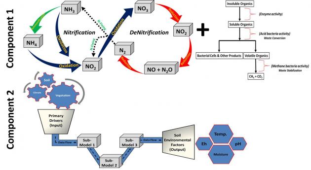
What Is the DNDC Model?
The DNDC (DeNitrification and DeComposition) model was developed for quantifying N2O emissions from agricultural soils in the late 1980s (US EPA, 1995). By including fundamental bio-geochemical processes of carbon and nitrogen transformations, DNDC was extended to model soil C sequestration and other trace gases (e.g., methane, nitric oxide, ammonia etc.) in the early 1990s.
DNDC consists of two components. The first component entails three sub-models and converts primary drivers (i.e., climate, soil, vegetation and anthropogenic activity) to soil environmental factors (i.e., temperature, moisture, pH, Eh and substrate concentration gradient). The second component consists of nitrification, denitrification and fermentation sub-models; and simulates production/consumption of N2O, NO, N2, NH3 and CH4 driven by the modeled soil environmental conditions [see graphic below]. With the bio-geochemical reactions embedded in the model framework, DNDC can predict the turnover of soil organic matter and the consequent trace gas emissions and nitrate leaching losses.
Feed ingredients
With input from industry and academic experts, our feed ingredient database was revised to better capture the expected range of ingredients typically available to producers in the US. Carbon, water and land footprint data as well as nutritional characteristics for the NRC growth equations were compiled for each feed ingredient. Economic models, that estimate the cost of feed, manure handling, utilities (water, electricity, gas, propane and diesel), dead animal disposal and immunocastration were integrated into the model. Capital costs are not considered. We are conducting cost benefit analyses on combinations of operations, manure management and dietary feeding systems aimed at reducing GHG emissions. These will help identify incentives to minimize mitigation strategy cost. Routines have been developed that will allow the user to download a set of updated prices for utilities and major feed ingredients.
DeNitrification and DeComposition (DNDC) Model (Soil)
The DeNitrification and DeComposition (DNDC) model requires numerous weather and site inputs, many of which are output from the environmental calculator, and others which require site-specific geographical characteristics (e.g., soil type). We analyzed the agricultural area of each continental-US county using agricultural classes from the 2013 NASS Cropland Data Layer. For each county, we assigned the mean latitude/longitude of all agricultural pixels as the agriculture-weighted centroid from which representative weather data will be extracted.
County soils data are derived from the NRCS General Soils Map (STATSGO). We derived the spatial intersection of STATSGO soil polygons with county boundaries. We summarized top soil data for each soil polygon from 0 to 10cm depth for clay fraction (a proxy for soil texture), bulk density, organic matter fraction (to estimate soil organic carbon, SOC), and pH. Modeled results will be based on either the comprehensive set of soil polygon attributes or a representative distribution of soil attributes for each county (depending on timing and available computing power).
Summary
The model will enable the user to find hot spots in their emissions profile, evaluate the effects of operational changes, and estimate the emissions from facilities during the design stage. The further addition of an operational economic model will provide the ability to perform cost/benefit analyses of practices that can change impact GHG emissions (see video).
Work will continue on this project through Spring, 2016.
Figure 1. Diagram of the DeNitrification and DeComposition (DNDC) model
Why Does This Matter?
The environmental footprint model, with improved algorithms for manure management, economics, and animal performance provide high resolution and flexible decision support for the swine industry. The model enables users to identify hot spots in their emissions and water/land use profiles, evaluate the effects of operational changes, and estimate the emissions from facilities during the design stage. The further addition of an operational economic model enables cost/benefit analyses.
These enhancements support evaluations of dietary energy, protein, and amino acid content for much of the life cycle and immunocastration and the use of ractopamine during the growth cycle. They also allow assessment of the performance, economic, and environmental impact of transient health events during the growth cycle with respect to whole farm operation.
The use and impacts on land and soils, air, water, and greenhouse gases all make up the environmental footprint of pork production. This section highlights many different aspects of pork production and how those impact emissions of greenhouse gases and other aspects of environmental impact.
Thermal Conversion of Animal Manure to Biofuel – Go to archive… (February, 2014)
Life Cycle Assessment Modeling for the Pork Industry – Go to archive…. (July, 2012)
Producer Association Efforts to Address Carbon Footprint (Pork and Poultry) – Go to archive… (June, 2012)
Research Summaries
a five-year project examining different aspects of the environmental footprint of pork production was recently completed. This project looked at feed rations, animal health, and manure management to provide data for integration into a comprehensive
Greenhouse gases and their contributions to climate change are some of the most studied topics in animal agriculture right now. What greenhouse gases are emitted by agriculture? How much is emitted in comparison to other industries?
Farmers, Ranchers, and Ag Professionals
Check out the self-study module “Greenhouse Gases and Agriculture“. When completed, you can receive a certificate or submit your completion for continuing education credits.
Teachers, Extension
The following materials were developed for teachers and educators to use in their classrooms and programs. The target age range is high school, jr. college and beginning farmer groups.
Instruction Guide (Lesson Plan): Includes links to additional information, connections to national agriculture education standards (AFNR Career Content Cluster Standards), application to Supervised Agricultural Experience (SAE) projects, activity and science fair ideas, sample quiz/review questions, and enrichment activities. PDF format (0.5 MB; best if you want to use it as-is) | RTF format (60 MB; best if you want to modify the file)
Western Region Animal Agriculture and a Changing Climate Extension Project
Our overall goal is for Extension—working with partner organizations—to effectively inform and influence livestock and poultry producers and consumers of animal products in all regions of the U.S. to foster production practices that are environmentally sound, climatically compatible, and economically viable.
Integrated Farm System Model (IFSM) and Dairy Gas Emissions Model (DairyGEM) – training presentation by Al Rotz.
Education received through either of these comprehensive model evaluations will lead to the development of more sustainable dairy and beef production systems.
The IFSM (Integrated Farm System Model) is a tool for evaluating environmental and economic effects of different farm management scenarios. The user enters information on cropping practices, facilities, equipment, the herd and other farm parameters. Sample farms of various sizes and types are provided with the model software to provide a starting point. Information generated by the model includes crop yields, feed production and use, animal production, manure handled, production costs and net return to management. The model’s environmental outputs include average annual soil balances of N, P, K and C, erosion of sediment, P runoff, nitrate leaching, emissions of ammonia, hydrogen sulfide and greenhouse gases, and the carbon footprint of the feed, animal weight or milk produced.
The Dairy Gas Emission Model (DairyGEM) is an educational tool that predicts ammonia and hydrogen sulfide volatilization, GHG emissions, and the carbon footprint of the milk produced. DairyGEM is used to study the interacting effects of management changes on major emission sources from feed production to the return of manure back to the land.
Dr. Al Rotz is an agricultural engineer at the USDA-ARS Pasture Systems and Watershed Management Research Unit in University Park, PA. His work focuses on the development and use of models to evaluate the performance, environmental impact and economics of alternative technologies and management strategies applied to integrated farming systems for dairy or beef production.
IFSM and DairyGEM Tool Training Presentation
(If one of the video windows is blank, please refresh the page.)
If you are interested in specific segments of the entire video tool training above for either IFSM or DairyGEM, please refer to the separate video segments below.
SEGMENT 1:
Introduction to both the Integrated Farm System Model (IFSM) and Dairy Gas Emissions Model (DairyGEM)
SEGMENT 2:
IFSM tool training (using dairy as an example)
**IMPORTANT Note: this segment also supports the use of DairyGEM
SEGMENT 3:
IFSM beef example and dairy example
SEGMENT 4:
DairyGEM Tool Training
***Note: for further instruction related to DairyGEM use, please refer to Segment 2
DeNitrification-DeComposition (DNDC) Model
DNDC (i.e., DeNitrification-DeComposition) is a computer simulation model of carbon and nitrogen biogeochemistry in agro-ecosystems. The model can be used for predicting crop growth, soil temperature and moisture regimes, soil carbon dynamics, nitrogen leaching, and emissions of trace gases including nitrous oxide (N2O), nitric oxide (NO), dinitrogen (N2), ammonia (NH3), methane (CH4) and carbon dioxide (CO2). In order to download the DNDC model files you will need to register and provide a valid email, as well as your affiliation and intended use. After registration and confirming your email you will be able to download the files from the DNDC Model Download page.
On the Download page, you will find 3 simulation models of interest.
The DNDC model – A computer simulation model for predicting crop yield, soil carbon sequestration, nitrogen leaching, and trace gas emissions in agro-ecosystems.
The Manure -DNDC Model- Ac computer simulation for predicting GHG and NH3 emissions from manure systems.
US Cropland GHG Calculator- A decision support system for quantifying impacts of management alternatives on GHG emissions from Agro-ecosystems in the U.S.
Manure and Nutrient Reduction Estimator Tool (MANURE Tool)
The MANURE Tool provides a system to quantify methane and and other GHG emission reductions and the environmental benefits of renewable energy produced by digesters at dairy and swine operations. The tool is based upon a full and accurate assessment of baseline conditions at the animal feed operation, which is a key element of the emission reduction calculation. This tool can be used to assess the quantity of emission reductions associated with implementation of specific technologies and/or practices. More information about the tool can be found on the Manure and Nutrient Reduction Estimator site.
COMET-FARM
The COMET-FARM tool is a whole farm and ranch carbon and GHG accounting and reporting system. It is intended to help users account for the carbon flux and GHG emissions related to their farm and ranch management activities, and help them explore the impacts to emissions of alternative management scenarios. The tool guides the user through describing the farm/ranch’s management practices including alternative future management scenarios. Once complete, a report is generated comparing the carbon changes and GHG emissions between current management practices and future scenarios. More information about COMET FARM can be found on the COMET-FARM site.
Farm Smart
Farm Smart is designed to give producers the ability to access and mitigate their environmental profile, track and measure their progress, plan for future improvements and report outcomes of practice changes to customers, community members, regulators and other stakeholders. The system features 3 tools: the Farm Smart Environmental Calculator, the Farm Smart Farm Energy Efficiency tool, and the Farm Smart Decision Support tool. Go to the Farm Smart site to download these tools and for more information.
Webcast Presentations
Fact Sheets
Regional Information
United States Global Change Research Program (USGCRP) Information:
(Hint: These links may take a few minutes to load. If you get a black screen and there is a note on the bottom task bar that says “done”, scroll down a little.)
Newsletters
Fill out the form below to sign up for the Western Region E-Newsletter
This online course is free and was developed to answer questions that the livestock and animal agriculture industry is facing related to climate. Nationwide, producers and stakeholders are asking questions about climate change: Is it happening? Are unusual weather patterns and events becoming more frequent? Should we be planning and managing for the future? Where can we get un-biased information that serves the livestock and ag community?
This online course will provide valuable information from which to feel confident in answering these frequent questions. Also, the online platform eliminates the extra travel expense for professional development.
Students that take this course will learn about the areas of climate and weather trends, impacts, adaptation, mitigation, policy, climate science and effective communication. Upon completion, they can receive CEUs from multiple professional societies.
Or please contact Liz Whitefield at e.whitefield@wsu.edu if you have any questions.
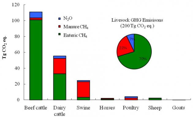
Agriculture is both a source and sink for greenhouse gases (GHG). A source is a net contribution to the atmosphere, while a sink is a net withdrawal of greenhouse gases. In the United States, agriculture is a relatively small contributor, with approximately 8% of the total greenhouse gas emissions, as seen below. Most agricultural emissions originate from soil management, enteric fermentation (the ruminant digestion process that produces methane), energy use, and manure management. The primary greenhouse gases related to agriculture are carbon dioxide, methane, and nitrous oxide. Within animal production, the largest emissions are from beef followed by dairy, and largely dominated by the methane produced in during cattle digestion.
U.S. greenhouse gas inventory with electricity distributed to economic sectors (EPA, 2013)
U.S. agricultural greenhouse gas sources (Adapted from Archibeque, S. et al., 2012)
Greenhouse gas emissions from livestock in 2008 (USDA, 2011)
Soil Management
Excess nitrogen in agriculture systems can be converted to nitrous oxide through the nitrification-denitrification process. Nitrous oxide is a very potent greenhouse gas, with 310 times greater global warming potential than carbon dioxide. Nitrous oxide can be produced in soils following fertilizer application (both synthetic and organic).
As crops grow, photosynthesis removes carbon dioxide from the atmosphere and stores it in the plants and soil life. Soil and plant respiration adds carbon dioxide back to the atmosphere when microbes or plants breakdown molecules to produce energy. Respiration is an essential part of growth and maintenance for most life on earth. This repeats with each growth, harvest, and decay cycle, therefore, feedstuffs and foods are generally considered to be carbon “neutral.”
Some carbon dioxide is stored in soils for long periods of time. The processes that result in carbon accumulation are called carbon sinks or carbon sequestration. Crop production and grazing management practices influence the soil’s ability to be a net source or sink for greenhouse gases. Managing soils in ways that increase organic matter levels can increase the accumulation (sink) of soil carbon for many years.
Animals
The next largest portion of livestock greenhouse gas emissions is from methane produced during enteric fermentation in ruminants – a natural part of ruminant digestion where microbes in the first of four stomachs, the rumen, break down feed and produce methane as a by-product. The methane is released primarily through belching.
As with plants, animals respire carbon dioxide, but also store some in their bodies, so they too are considered a neutral source of atmospheric carbon dioxide.
Manure Management
A similar microbial process to enteric fermentation leads to methane production from stored manure. Anytime the manure sits for more than a couple days in an anaerobic (without oxygen) environment, methane will likely be produced. Methane can be generated in the animal housing, manure storage, and during manure application. Additionally, small amounts of methane is produced from manure deposited on grazing lands.
Nitrous oxide is also produced from manure storage surfaces, during land application, and from manure in bedded packs & lots.
Other sources
There are many smaller sources of greenhouse gases on farms. Combustion engines exaust carbon dioxide from fossil fuel (previously stored carbon) powered vehicles and equipment. Manufacturing of farm inputs, including fuel, electricity, machinery, fertilizer, pesticides, seeds, plastics, and building materials, also results in emissions.
To learn more about how farm emissions are determined and see species specific examples, see the Carbon Footprint resources.
To learn about how to reduce on-farm emissions through mitigation technology and management options, see the Reducing Emissions resources.
Additional Resources
Additional Animal Agriculture and Climate Change Resources
The Earth’s climate system is composed of a number of interacting components. The main driver is the sun whose energy is by far the main source of heat for Earth. The sun does not heat the Earth’s atmosphere directly but rather its energy passes through the atmosphere and heats the surface of Earth. The surface then heats the atmosphere from below. If the Earth did not lose heat to space, it would continue to heat up as energy is supplied from the sun. To maintain a fairly constant temperature the Earth must lose as much heat to space as it gains. Clouds, along with naturally occurring carbon dioxide in the atmosphere, prevent some of this heat from escaping and thus warm the Earth. Without these components in the atmosphere the temperature of the globe would be about 60°F colder than it is today. Besides blocking the loss of heat from Earth to outer space, clouds can also reflecting sunlight back to space. This reflected energy is unavailable to heat the Earth.
All of the components of the climate system interact. For example, during ice ages, the growth of ice sheets is triggered by a reduction in the amount of energy reaching the Earth from the sun. As the ice sheets grow, forest and soil covered surfaces, which normally absorb (and therefore are warmed by) solar energy, are replaced by ice. Ice reflects most of the sun’s energy making it unavailable to warm the surface. Therefore the growth of the ice sheets contributes to further cooling of the planet. This is known as a positive feedback, since the cooling due to the reduction in solar energy is enhanced by the ice sheet. The same positive feedback results from global warming, as the extent of the ice sheets diminishes, more soil and potentially forest is exposed. These surfaces absorb more heat than the ice covered areas and hence the warming is enhanced.
Natural forces that effect the climate system
Ice ages are just one example of how the Earth’s climate varies through time. Other variations can be caused by:
Natural fluctuations in the sun’s intensity. The amount of energy emitted by the sun is not constant. Changes in its intensity are typically small (a few tenths of a percent), but can influence temperatures on Earth if they occur over an extended period of time.
Volcanic eruptions. Violent volcanic eruptions like Mt. Pinatubo in 1991 inject sulfur dioxide into the upper atmosphere. This compound is highly reflective to sunlight. Thus its presence in the upper atmosphere prevents a portion of the sun’s energy from reaching the Earth. Once in the upper atmosphere, these compounds can exist for several years following the eruption.
Shorter-term cycles like El Nino. The oceans and atmosphere work together to influence climate. Natural oscillations in ocean currents, the location of the warmest or coldest ocean temperatures, etc. can influence atmospheric circulation patterns. El Nino is an example. In this case the pool of warm water that usually resides in the western tropical Pacific Ocean migrates east. This changes the atmospheric circulation pattern in the tropics which influences global weather patterns.
Human factors affecting the climate system
Increase in greenhouse gases. Carbon dioxide and water vapor are both natural components of the Earth’s atmosphere. These gases, along with methane, nitrous oxide and ozone are termed greenhouse gases (GHGs) because of their ability of absorb some of the energy that the Earth emits to space and reradiate it back to the surface. Prior to industrialization, the Earth’s atmosphere contained about 280 parts per million of carbon dioxide (280 CO2 molecules for every 1,000,000 molecules in the atmosphere). This carbon dioxide was maintained in the atmosphere via volcanic and biological activity.
This graph shows long-term trends in carbon dioxide, the primary anthropogenic (humanmade) greenhouse gas (other greenhouse gases include methane and nitrous oxide). In all but the most recent part of the record the data were obtained from analyzing air samples trapped in
ice cores. Direct measurements have been made since the mid 1950s and fit nicely with the ice core record. Carbon dioxide concentration was very constant prior to 1860. After 1900 the concentrations all increase exponentially.
What causes these increases?
Fossil fuel burning releases about 6 billion tons of carbon each year into the atmosphere.
Methane from agriculture, livestock, landfills and industry has increased by 133%.
Nitrous oxide from agriculture and industry has increased by 15%.
Changes in land use and land cover release 1 billion tons of carbon annually plus other gases.
Land use changes include deforestation and urbanization. Deforestation influences the climate in two ways. 1) Trees are sinks for atmospheric carbon dioxide. They remove CO2 from the air and store it as vegetative matter. Fewer trees mean less CO2 is pulled from the atmosphere. If the trees are subsequently burned, the CO2 is added back to the atmosphere. 2) Removal of the trees changes the character of the land surface; this changes the amount of solar energy that is absorbed by the surface, evaporation, etc. Urbanization is similar to deforestation. Urban areas tend to absorb and hold more heat than vegetated surfaces. Thus cities are typically warmer than rural environments.
Recent Climate Change
When the concentration of greenhouse gases is increased (and everything else in the climate system, like the amount of clouds, is held constant) less of the Earth’s energy escapes to space. As a result the temperature of the Earth must rise.
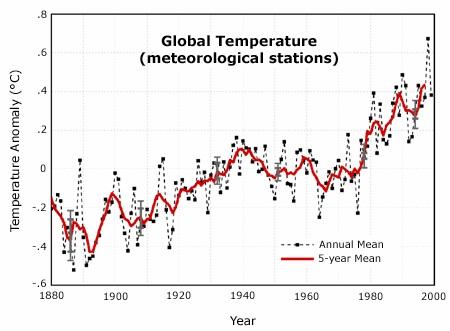
Temperature. Over the last 100 years, instrumental records indicate that the average temperature of the Earth has risen by nearly 1°F (0.5°C). The increases are most pronounced in polar regions of the Northern Hemisphere. In Alaska, temperatures have risen about 2.8°F (1.5°C) over the last century. Across the globe, the increase in temperature tends to be largest in winter, but still significant during the other seasons. Night time temperatures have risen faster than values observed during the day. U.S. temperatures have risen by 0.9°F over the past100 years. Within the past 25 years, U.S. temperatures increased 1.6°F.
Precipitation. Although average precipitation across the globe has not changed dramatically, a change in the character of precipitation has been observed in many parts of the world. The observed trends suggest a shift from more frequent moderate rainfall events to more infrequent heavy rainfall events. Since the period of time between rainfall events increases, drought may become more prevalent. But since the rain events that do occur can be quite heavy, the increased risk of flooding is also a concern. Clearly this change in the character of precipitation has implications for water resource and irrigation decisions.
Predictions
CO2 Levels. In order to project future climate conditions, scientists must predict what the world will look like politically, economically and environmentally in 100 years. Given the uncertainty in such predictions, scientists have developed a range of scenarios of future greenhouse gas emissions. These range from a fossil-fuel intense society that undergoes rapid economic growth and experiences a modest increase in population. In this case atmospheric CO2levels increase to four times their pre-industrial values by 2100. A business-as-usual scenario…continuing the present trend in greenhouse gas emissions … leads to a similar increase in CO2 levels by 2100 (A2 in the figure below).
More environmentally-friendly scenarios, with reductions in fossil fuel usage, also lead to increases in atmospheric CO2 concentration. This results from the lifetime of CO2 in the atmosphere (about 100 years). Thus today’s CO2 emissions are not removed from the atmosphere until 2106. Even the most environmentally friendly emission scenarios lead to an increase in atmospheric CO2 concentration over the next 100 years, to about double preindustrial levels (B1 in previous figure).
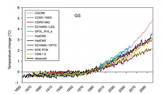
Temperature. Many climate models exist. They all rely on the same physics, but differ in the ways in which variables like clouds are parameterized. The “art” of climate modeling is how processes that can not be well represented by the physics of the models are accounted for. All models experience the same increase in greenhouse gas concentration. They all show a warming by 2100. The only difference is the magnitude of the warming. Here model warming estimates range from 1.5 to 5.0°C by 2100.
Significance. At first glance a degree or two or even five degrees of “global warming” does not seem like a big deal. However when averaged over the globe, this change is quite substantial. From the height of an ice age to the intervening interglacial period (like today) the globe’s temperature changes by about six degrees. The more modest climate model projections are that by 2100, increase global temperature will be about a third of that associated with the ice age cycle. Keep in mind that for ice ages, this six-degree change occurs over 100,000 years. We
expect to see a 2-3 degree change over 100 years!
Precipitation. The figure below shows how precipitation changes will vary geographically by 2100. Some locations (primarily in subtropics) show decreases in precipitation (orange and gold areas in the figure below). Large areas of the middle latitudes and tropics see increases in
precipitation.
Summary
Over the last century the concentration of greenhouse gases in the Earth’s atmosphere has increased markedly. CO2 levels in the atmosphere have not been this high for hundreds of thousands of years. In isolation this change must result in a warming of the Earth’s temperature. Over this same time period climate observations indicate that the global temperature has increased by about 1°F. Although changes in average precipitation have been small (on the order of 1-2%), rain gauge records show that the character of precipitation events has changed. Heavy rainfall events have become more frequent over the last half century.
It is unlikely that the emission of carbon dioxide into the Earth’s atmosphere will slow in the near future. In fact, most projections indicate increased carbon dioxide emissions into the middle to late part of the 21st century. This continued increase will likely lead to additional increases in temperature, with most models projecting rises of between 1.5 and 5°C. Although the exact magnitude of changes in precipitation are uncertain, there is reason to believe that precipitation events will become more variable, leading to increases in both the frequency of floods and droughts.
The Natural Resources Conservation Service (NRCS) has begun developing online courses in three curriculum tracks: air quality, energy, and climate change. Air Quality, Climate Change, and Energy is the lead-in to the three tracks.
The courses are designed for all Natural Resource Conservation Service (NRCS) employees, but particularly for State Air Quality and Energy Contacts, conservation planners, partnership employees, and conservation technical assistance providers to assist them in integrating air quality, energy and climate change into conservation planning and programs. Although these courses were developed specifically for NRCS employees, the information contained in them may also be useful to NRCS partners and others associated with conservation in agriculture.
Other courses are either in development or are being planned to supplement the learning modules for each of these curriculum tracks
Air Quality, Climate Change, and Energy
Turkey production. Photo courtesy USDA NRCS.
Upon completion of the course, participants will be able to:
Define air quality, climate change, and energy as they relate to the NRCS mission and explain how they are interrelated
Explain the importance of these issues for land managers and NRCS itself
Recognize how soil, water, air, plants, animals and human activity all affect, and are affected by, energy and climate change
Identify examples of how air quality, climate change, and energy concepts apply to agricultural conservation
List and locate additional resources that can be used to expand knowledge of these topics
Course Link. Air quality is already a functional part of the NRCS conservation portfolio (the first ‘A’ in SWAPA+H). Climate change and energy are now becoming significant considerations in conservation planning. This course will provide a broad overview of these three topics, and how they are related to each other and SWAPA+H components. Students will learn how agricultural activities can contribute to air emissions, sequester carbon, manage greenhouse gas emissions, and better conserve energy. The course also will provide examples of addressing these issues via NRCS planning and programs. 90 minutesGo to Air Quality, Climate Change, and Energy….
Why Should We Care About Air Quality?
Upon completion of the course, participants will be able to:
State why air is an important natural resource
Explain why it is important to take a holistic approach to conservation planning
List the major reasons why NRCS addresses air quality and atmospheric change
Identify several agricultural activities that can release air emissions
Describe various reasons for land managers to address air quality and atmospheric change
Identify the role of NRCS employees in addressing air quality and atmospheric change
Course link. As the first “A” in SWAPA+H, air is an important natural resource that is vital to life. Although our agency has addressed issues related to air quality and atmospheric change since its formation, these issues have not been a traditional focus area for the NRCS in most locations. As our partners and the public have begun placing a larger emphasis on air quality and atmospheric change issues, NRCS has needed to develop the technical expertise for integrating conservation of the air resource into our assistance portfolio.
This course will provide a broad overview of air quality and atmospheric change and begin to equip NRCS conservationists and our partners with the knowledge and confidence to address air-related resource concerns. 30 minutes.Go to Why Should We Care About Air Quality?…
Manure management system for a swine farm. Photo courtesy USDA NRCS.
Air Quality Resource Concerns
Upon completion of the course, participants will be able to:
Identify the four primary air quality resource concerns and the emissions that contribute to these concerns
Identify the effects of particulate matter, ozone precursors, and odors on air quality
Discuss greenhouse gases as an atmospheric change issue
Derive potential solutions to reduce agricultural emissions of particulate matter, ozone precursors, odors, and greenhouse gases
List and locate additional resources that can be used to expand knowledge of these topics
Course link. The NRCS utilizes the concept of “resource concerns” in conservation planning. There are four broad categories of air-related resource concerns: particulate matter, ozone precursors, odors, and greenhouse gases and carbon sequestration. This course provides an overview of each of these four air quality resource concerns and how they can most effectively be addressed in the NRCS planning framework. Principal air emissions from agricultural operations are discussed, and how each of these is related to one or more of the air resource concerns. Finally, a variety of mitigation strategies are presented for managing emissions and improving these four air quality concerns. 50 minutesGo to Air Quality Resource Concerns…
Air Quality and Animal Agriculture
Upon completion of the course, participants will be able to:
Identify the primary reasons that animal production operations are currently the main focus when discussing air quality issues in agriculture
Identify the primary air emissions from animal production operations and describe how these emissions are generated, emitted, and transported
Identify NRCS options for mitigating air emissions from animal production operations
When discussing air quality issues in agriculture, animal production operations are typically the primary focus for mitigation and regulation. This course will introduce the air emissions associated with animal operations and provide information on how NRCS can help producers mitigate these emissions. 60 minutes Go to Air Quality and Animal Agriculture…
Greenhouse Gases and Carbon Sequestration
Upon completion of the course, participants will be able to:
Explain the greenhouse effect
Discuss the characteristics of sunlight and earth’s radiation balance
Determine how changes in greenhouse gas emissions can influence global climate change
Identify methodologies in which agricultural and natural resource systems can mitigate greenhouse gas emissions and effects
Given a scenario, explain the importance of a holistic approach to the reduction of greenhouse gas emissions
Course Link Climate change and carbon offset trading have gained great interest in many parts of the agricultural community over the past few years. But why should we as NRCS conservationists be interested in these issues? Conservation systems that we design and help implement can often have a positive influence on the emission or storage of gases which, when in the atmosphere, can affect climate change. This course shows the importance of greenhouse gases to life on earth, the potential negative consequences of increasing greenhouse gas concentrations in the atmosphere, agricultural sources of greenhouse gases, and potential methods in which agriculture can reduce its net emissions of greenhouse gases to the atmosphere. 60 minutesGo to Greenhouse Gases and Carbon Sequestration…
Why Do We Care About Energy?
Upon completion of the course, participants will be able to:
Describe why energy costs and energy security are so important to land managers.
Describe environmental impacts of fossil fuel exploration, production and use.
Describe energy opportunities available to land managers and NRCS
Course Link While energy has not traditionally been addressed in the NRCS planning process, it is receiving unprecedented attention in the national and international news. This short course provides insight into why energy issues are important to agriculture and the nation. It gives participants the opportunity to explore how our energy choices can impact NRCS and the natural resources we work to conserve. 30 minutes Go to Why Do We Care About Energy?…
Upon completion of the course, participants will be able to:
Describe basic terminology and energy concepts.
Identify non-renewable and renewable sources of energy and describe their origins, benefits and uses
Explain life cycle analysis and it relevance to comprehensive energy planning
Describe agriculture’s role in utilizing renewable energy alternatives
Course Link Understanding energy basics is fundamental to effective energy conservation planning. This course establishes a technical foundation to prepare NRCS planners to incorporate energy considerations into conservation plans. It provides general background on the fundamental principles behind energy issues in agricultural settings. 90 minutesGo to Energy Basics…
Why Do We Care about Climate Change?
At the completion of this course, students will be able to:
Understand climate change and its key drivers
Explain the impacts of climate change on agriculture and natural resources
Differentiate mitigation from adaptation
Discuss NRCS’ role in helping land managers and owners in mitigating and adapting to the impacts of climate change
Course link. Climate plays a key role in conservation planning, natural resource management and agricultural production. Changes in climate can have significant impacts on managing and protecting agricultural and natural resources. NRCS is educating its employees and partners about climate change, and communicating climate change impacts to NRCS customers. Understanding climate change and its impacts will help NRCS assist private landowners, producers, and land managers cope and adapt to changing climate.
This course discusses climate change and related concepts, the impacts of climate change on agriculture and natural resources, and NRCS’ role in helping private land owners and land managers address climate change mitigation and adaptation through conservation planning. 30 minutes. Go to “Why Care About Climate Change?”
Course link: This course provides an introductory discussion of environmental credits, environmental credit trading, and market-based approaches providing environmental and economic benefits.
At the completion of this course, students will be able to:
Understand environmental credit trading
Identify markets for environmental credits
Explore the benefits and costs of participating in markets
Understand how different environmental practices can produce various environmental credits
Outline various ways agricultural producers can benefit from environmental credit trading
Explain how producers can participate in environmental credit trading
Greg Zwicke, P.E.
Air Quality Engineer
Air Quality and Atmospheric Change Team
USDA-NRCS, WNTSC
2150 Centre Ave.
Building A, Suite 231
Ft. Collins CO 80526
To provide the best experiences, we use technologies like cookies to store and/or access device information. Consenting to these technologies will allow us to process data such as browsing behavior or unique IDs on this site. Not consenting or withdrawing consent, may adversely affect certain features and functions.
Functional
Always active
The technical storage or access is strictly necessary for the legitimate purpose of enabling the use of a specific service explicitly requested by the subscriber or user, or for the sole purpose of carrying out the transmission of a communication over an electronic communications network.
Preferences
The technical storage or access is necessary for the legitimate purpose of storing preferences that are not requested by the subscriber or user.
Statistics
The technical storage or access that is used exclusively for statistical purposes.The technical storage or access that is used exclusively for anonymous statistical purposes. Without a subpoena, voluntary compliance on the part of your Internet Service Provider, or additional records from a third party, information stored or retrieved for this purpose alone cannot usually be used to identify you.
Marketing
The technical storage or access is required to create user profiles to send advertising, or to track the user on a website or across several websites for similar marketing purposes.
 Algal biomass offers many advantages over traditional energy crops; algal biomass generates higher yields and requires smaller land area than other energy crops. In addition to biomass production for potential biofuel feedstock generation, algal growth systems can also act as tertiary treatment systems for wastewater. Algal growth can dramatically reduce nitrogen and phosphorus from wastewater. Unlike conventional open pond and photo-bioreactor systems, periphytic systems (e.g., algal turf scrubbers) generally involve the polyculture of micro-algae, which does not require specialized conditions. While algal turf scrubber systems are traditionally used for water treatment, they are also capable of generating high biomass yields.
 Many technologies being considered incorporate some type of manure separation to concentrate manure solids, nutrients, and energy content. An LCA study in Denmark showed that energy recovery (incineration, gasification, and anaerobic digestion) had lower GHG emissions than traditional land application of swine manure. Other studies point to the complexities of manure management system design options in relation to GHG emissions. This portion of the project will quantify the effect of various solid separation approaches on the chemical composition of the manure generated by the feed trials at the University of Arkansas facilities during this project ,and generate the necessary manure solids for the thermo-chemical conversion portion of this project. Design and construct a pilot scale mobile solids separation system (see image below) is currently approaching completion and anticipated to be ready to begin trial calibrations soon.
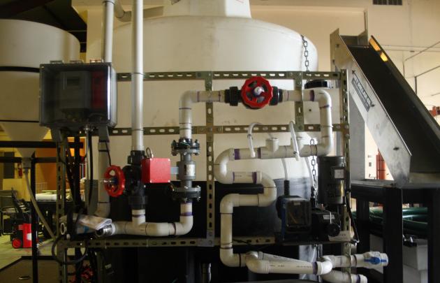
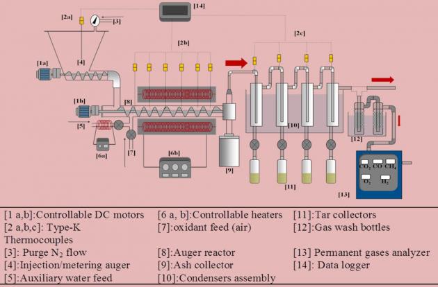

 Maximizing feed grade amino acid (FGAA) use and reducing dietary crude protein in swine diets has been shown to dramatically reduce nitrogen excretion in both nursery and growing/finishing swine which could substantially reduce nitrous oxide (N
 Our working hypothesis is that immune activation, from clinical and subclinical disease, reduces growth performance and concomitantly increases nutrient excretion and subsequent
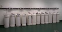
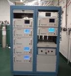

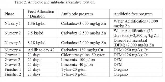
 Project Objectives